Calibrating a Mosaicked Spectral Line Dataset
This page assumes you have converted your data from native MIRIAD format to a CASA measurement set (MS). It also assumes that you have put the filename of the original MS into a global CASA variable, e.g.,
# In CASA
msdir='./'
project='c0xxx'
msfile=msdir+project+'.ms'
Examining your data
You'll need some information about the IDs that CASA assigns to your calibrators, sources, and antennas. So if you haven't yet done so,
# In CASA
listobs(vis=msfile)
You will want to know:

- The FieldId of each of your sources and calibrators.
- The SpwId of each spectral window you want to calibrate.
- The Name (or station, but not the ID ) of your reference antenna.
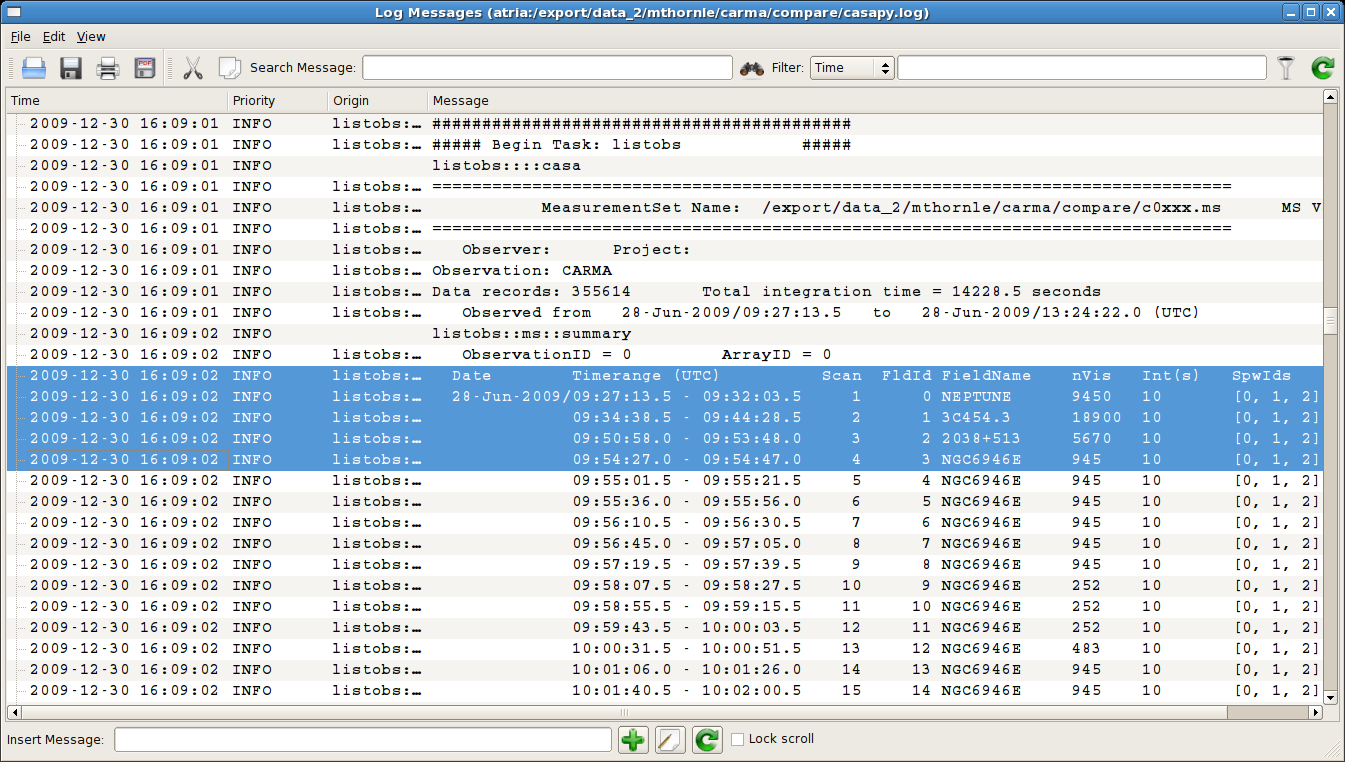
Near the beginning of the listobs output, you will find the first listing of FldId numbers. In this case, the flux calibrator (NEPTUNE) is assigned FldId=0, the bandpass calibrator (3C454.3) is assigned FldId=1, the phase calibrator (2038+513) is assigned FldId=2, and the mosaicked source fields are assigned FldId 3 through 51 (that's field='3~51' in python).
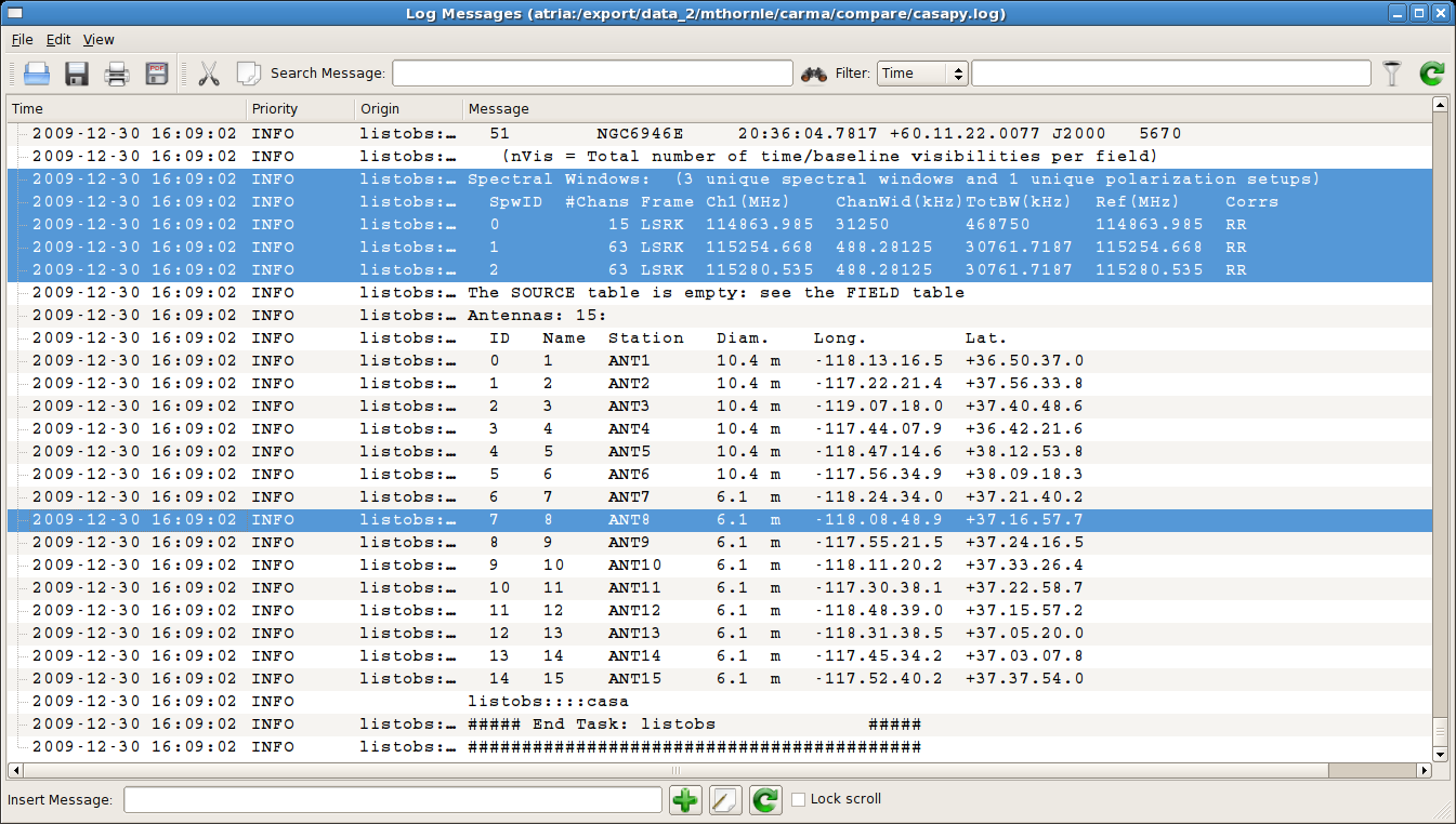
Near the end of the listobs output, you will find listings of the properties of the observed spectral windows, and the locations of the antennas. In this case, the narrowband windows are assigned to SpwID of 1 and 2, and they each have 63 channels. The reference antenna is Antenna 8, which unfortunately here is named '8'. For unambiguous antenna selection, ideally the Name (which CASA searches first) should have text in it; if it does not, you may want to use the unambiguous Station name of 'ANT8' to ensure that CASA chooses the right antenna.

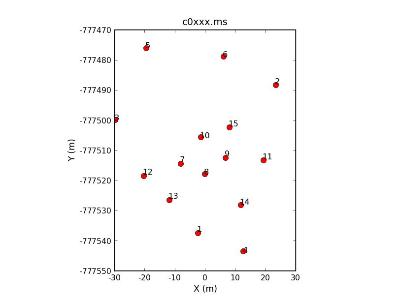
It's not particularly clear, without a closer look at this output, which antenna you should use as the reference antenna. You can get this information using plotxy. The following command
# In CASA
plotxy(vis=msfile,xaxis='x')
will display the physical layout of the antennas.

You can see antenna 8 near the middle of the CARMA array.
Calibrating your data
Before running your calibration, it's a good idea to run the following command:
# In CASA
clearcal(vis=msfile)
If this is the first time you've calibrated, clearcal won't do much, but it will initialize table columns that might be missing from the import step (you may see some output to the log screen to this effect). If you are trying a new calibration, this command ensures your data returns to their original state. So it can't hurt you, and can help.
Calibration in CASA consists of creating calibration tables, and then applying them as needed. Here, we step you through bandpass and amplitude calibration, and then indicate how to apply them to your source data.
Bandpass calibration
The following command (bandpass) will create a bandpass calibration table (caltable=) using the specified bandpass calibrator (field=FldId) and reference antenna (refant), in the same directory as the data are found. No prior gain tables are applied in this step, but they could be if it were necessary (just fill in the appropriate information for gaintable and gainfield).
# In CASA
default('bandpass')
bandpass(vis=msfile,caltable=msdir+proj+'.bcal',gaintable='',gainfield='',
         interp='',field='1',spw='',gaincurve=False,
         bandtype='B',solint='inf',refant='ANT8',
         solnorm=True)
Amplitude calibration
Since 3C454.3 is strong enough to serve as both bandpass and flux calibration, we will use it for both in this example. As in AIPS the task setjy is used to provide source information for objects of known flux and distribution. However, 3C454.3 is not currently known as a flux calibrator, so a source flux density will need to be provided explicitly (e.g., using the CARMA flux calibrator database). For example, if you determine that your calibrator is a point source with a flux density of 6.6 Jy, you would add this information into your dataset using the following command:
# In CASA
setjy(vis=msfile, field='1',fluxdensity=[6.6,0.,0.,0.], spw='0~2')
The task gaincal can then be used to determine the appropriate gains to be applied as a function of time. Here, we include both the bandpass calibrator (nice and strong, but not observed often: field='1') and the phase calibrator (weaker, but observed periodically throughout the observations: field='2'). In this example, the wideband data (spw='0') is used for better signal-to-noise, and I have used the station title of the reference antenna (refant='ANT8') to unambiguously identify it.
The bandpass calibration table, specified here by gaintable, is accounted for prior to determining the gain table, so that the two calibrations remain separate. Note: neither the gain or bandpass calibration is actually applied to the data here; both calibrations will need to be applied after the fact, using applycal (see below).
# In CASA
gaincal(vis=msfile,caltable=msdir+proj+'.gcal',gaintable=msdir+proj+'.bcal',
        gainfield='1', field='1,2', spw='0',
        gaintype='G',minsnr=2.0, refant='ANT8', solint='inf', combine='')
Now that the gains have been determined, I can bootstrap the flux of 3C454.3 to the other sources, using fluxscale. This command uses the gain table (specified by caltable) and needs to be told which source is the reference source (3C454.3, so that reference='1').
# In CASA
fluxscale(vis=msfile,caltable=msdir+proj+'.gcal',
          fluxtable=msdir+proj+'.fcal', reference='1')
Note: All of the information from the gain table is contained in the flux table, so in the end, you will apply the bandpass and flux calibration tables in order to apply all relevant calibrations.
Applying your calibrations
Now that you have solutions for both bandpass and gain calibration, you can apply them to your data. Note that applycal does not operate on the raw data in this step, so you do not need to create a copy of the data before proceeding. Use of the command clearcal will return your data to a pristine state, if needed.
Applycal is quite powerful and very flexible, allowing you to apply multiple calibration tables, and calibrations from one spectral window to others. Here are two examples of applying calibrations, but these are still relatively simple. Consult the helpfile for applycal for a detailed explanation of how to use this command--note in particular the complex uses of the parameter spwmap.
In the first example, we apply calibrations to the bandpass/flux calibrator (3C454.3, field='1'). We apply both bandpass and flux calibration table. The order of entries in gainfield and spwmap are the same as for gaintable: in this case, it means that we take the bandpass calibration for 3C454.3 (gainfield=['1',...) and apply the solutions for each spectral window to the same spectral window for the other sources (spwmap=[[],...), but we take the gain/flux calibration of the same source (gainfield=...,'1']from the wideband channel (spw='0') and apply it to all spectra windows (spwmap=...,[0]]).
You would only want to do this if you wanted to image the bandpass/flux calibrator.
# In CASA
applycal(vis=catfile,field='1',spw='',
         gaintable=[msdir+proj+'.bcal',msdir+proj+'.fcal'],
         gainfield=['1','1'],spwmap=[[],[0]])
In this second example, we apply bandpass and flux calibrations to the rest of the sources (phase calibrator, field='2'; source, field='3~51'). In this case, we use the flux calibration information for the phase calibrator to apply to the source, as it has finer time sampling.
# In CASA
applycal(vis=catfile,field='2~51',spw='',
         gaintable=[msdir+proj+'.bcal',msdir+proj+'.fcal'],
         gainfield=['1','2'],spwmap=[[],[0]])
You're done calibrating! Now proceed onward to Imaging your Mosaicked Spectral Line Dataset.