ACA Simulation (CASA 3.3)

↵ Simulating Observations in CASA

To create a script of the Python code on this page see Extracting scripts from these tutorials.

ALMA 12m + ACA + Total Power

Multiple configurations, or an observation in one 12m configuration plus one ACA observation, or other combinations, can be simulated by running sim_observe for each, and then combining the Measurement Sets to run sim_analyze. Total power observations can be simulated either in an independent run of sim_observe, or along with an interferometric simulation. Note that if you simulate total power and an interferometric observation simultaneously with sim_observe, they must have the same set of pointing centers and the same integration and total time, which is probably not realistic. (For example it is generally recommended to observe a larger area by 1/2 primary beam in total power mode to combine with a 12m ALMA mosaic).

• Simdata version for CASA 3.3

Explanation of the script

Set sim_observe as current task

Reset all parameters to default, and then set the project name to m51c

# Set sim_observe to default parameters
default("sim_observe")
# Our project name will be m51c, and all simulation products will be placed in a subdirectory m51c/
project="m51c"

Specify sky model image

We'll use an Halpha image of M51 as an example model sky. Download from here and place in your working directory.

# Model sky = Halpha image of M51 
modelimage         =  "m51ha.fits"

Although the image has a world coordinate system, we want to override most of the parameters.

• We'll place the source in the southern hemisphere with the indirection parameter,
• set the pixel size to 0.1arcsec, effectively moving the galaxy further away (M51 itself would require a quite large mosaic, and in any case we need for the input model pixels to be significantly smaller than the synthesized beam that we'll be simulating, or else we won't be learning anything)
• set the frequency to 330GHz, and since its a 2D image we'll set the single "channel" width to be 50MHz, and peak brightness of 0.004 Jy/pixel - parameters plausible for observing an emission line in a galaxy.

# Set model image parameters:
indirection="B1950 23h59m59.96s -34d59m59.50s"
incell="0.1arcsec"
inbright="0.004"
incenter="330.076GHz"
inwidth="50MHz"

We need to decide where to point the telescope. The image is 2/3 arcsec in size, so we only need one pointing. We could put that in a text file ourself, or let simdata create the ascii pointing file for us.

setpointings       =  True
direction          =  "J2000 18h00m00.031s -22d59m59.6s"
mapsize            =  "0.76arcsec"

We do want to calculate visibilities in a measurement set: let's do a 20 min snapshot observation using the "out20" ALMA antenna configuration:

observe            =  True
totaltime          =  "1200s"

Use appropriate antenna configurations based on desired angular resolution (configuration 20 - alma.out20.cfg in this case - is the largest "compact" configuration)

# It might be helpful to confirm the alma.out20.cfg file exists in the path defined below
# If you have a problem, this might be the first thing to check, if you haven't already
repodir=os.getenv("CASAPATH").split(' ')[0]
antennalist        =  repodir+"/data/alma/simmos/alma.out20.cfg"

Deconvolve the visibilities back into an image

image              =  True
vis                =  "$project.ms"
imsize             =  [192, 192]

Specify number of iteration of cleaning task with proper threshold and weighting

niter              =  10000
threshold          =  "1e-7Jy"
weighting          =  "natural"

We'd like to calculate a difference and fidelity image, and see some diagnostics:

analyze            =  True

And see the array but not the UV coverage:

showarray          =  True
showuv             =  False

Plot both to the screen and the png files with lots of messages:

graphics           =  "both"
verbose            =  True
overwrite = True

Run simdata

# This commands CASA to execute simdata
simdata()

• Output results:

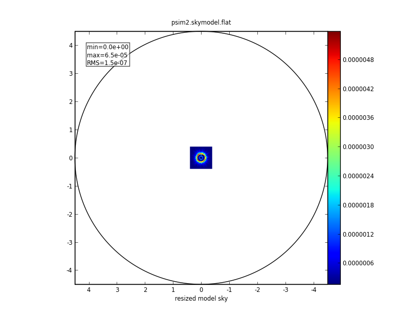
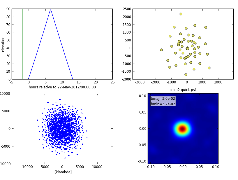
Input:	Predict:
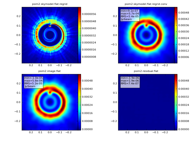
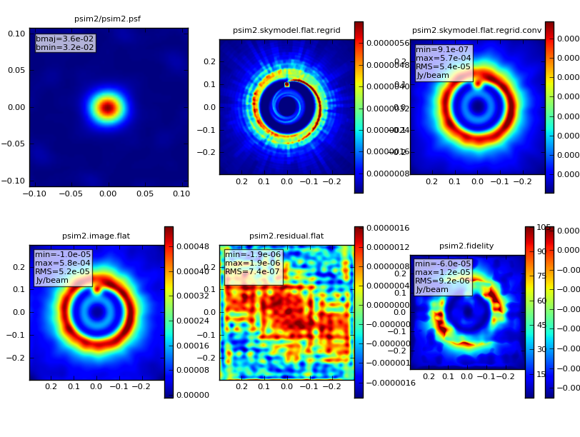
Image:	Analyze:

↵ Simulating Observations in CASA