NGC 5921: red-shifted HI emission 5.7.2
Overview
The technique used to calibrate and image continuum datasets generally applies to spectral line observations, except that an additional calibration step is required. Bandpass calibration flattens the spectral response of the observations, ensuring that spectral channel images are properly calibrated in amplitude and phase.
The following tutorial derives from an annotated script provided in the CASA Cookbook. The script is largely reproduced in sections and additionally annotated with figures and illustrations.
The data are included with the CASA installation.
Setting up the CASA Environment
Start up CASA in the directory you want to use.
# in bash
mkdir NGC5921
cd NGC5921
casapy
Now, in CASA, set up paths and global variables to facilitate the data reduction. These operations can be performed on-the-fly if you are reducing data interactively, but it's better to get them out of the way in the scripting environment.
import os
scriptmode = True

prefix = 'ngc5921.demo' # The prefix to use for all output files
# Set up some useful variables (these will be altered later on)
msfile = prefix + '.ms'
btable = prefix + '.bcal'
gtable = prefix + '.gcal'
ftable = prefix + '.fluxscale'
splitms = prefix + '.src.split.ms'
imname = prefix + '.cleanimg'
We'll use a python os command to get the appropriate CASA path for your installation. The use of os.environ.get is explained in the Appendix.
pathname=os.environ.get('CASAPATH').split()[0]
fitsdata=pathname+'/data/demo/NGC5921.fits'
Scripts are of course modified and repeated to the satisfaction of observer. To help clean up the bookkeeping and further avoid issues of write privileges, remove prior versions of the measurement set and calibration tables.
Tip: The first command in the following code block removes the measurement set. Depending on the size of the source data, refilling a measurement set can be time-consuming, and so you may want to consider editing a separate script that preserves the measurement set but skips the importuvfits command given below. This particular dataset is not very large and so refilling is fairly quick.
rmtables(msfile)
rmtables(btable)
rmtables(gtable)
rmtables(ftable)
rmtables(ftable)
rmtables(splitms+'*')
rmtables(imname+'.*')
rmtables(prefix+'.moments*')

# Final clean up of auxiliary files
os.system('rm -rf '+prefix+'*')
Import the Data
The next step is to import the multisource UVFITS data to a CASA measurement set via the importuvfits filler.
# Safest to start from task defaults
default('importuvfits')

# Set up the MS filename and save as new global variable
msfile = prefix + '.ms'

# Use task importuvfits
fitsfile = fitsdata
vis = msfile

saveinputs('importuvfits',prefix+'.importuvfits.saved')

importuvfits()
Saveinputs saves the parameters of a given command to specified text file, handy to debug a script and see what actually was run. Here, the parameters of importuvfits are saved to the file "ngc5921.demo.importuvfits.saved". Here's a listing of this file. Notice that it is executable with execfile in CASA (remove the # commenting symbol before importuvfits to have the execfile run the command).
CASA <71>: os.system('cat ngc5921.demo.importuvfits.saved')
taskname           = "importuvfits"
fitsfile           =  "/usr/lib64/casapy/30.0.9709test-001/data/demo/NGC5921.fits"
vis                =  "ngc5921.demo.ms"
antnamescheme      =  "old"
#importuvfits(fitsfile="/usr/lib64/casapy/30.0.9709test-001/data/demo/NGC5921.fits",vis="ngc5921.demo.ms",antnamescheme="old")
A Summary of the Data
We'll need to have a look at the observing tables to learn the calibrator and source names. The relevant command is listobs.

listobs(vis='ngc5921.demo.ms', verbose=True)
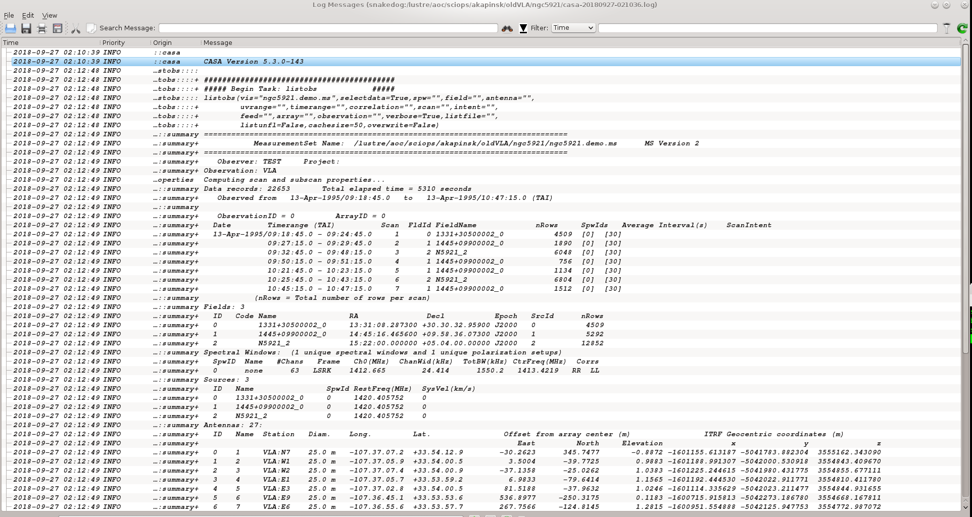
The output goes to the logger window; see the screenshot at right.
Tip: You can control the text size of the logger window using <ctrl>-A (smaller font) and <ctrl>-L (larger font).
A more complete listing of the listobs output follows.
INFO listobs	##### Begin Task: listobs            #####
INFO  	listobs::::casa
================================================================================
           MeasurementSet Name:  /DATA/ASHLESHA_2/NGC5921/ngc5921.demo.ms      MS Version 2
================================================================================
   Observer: TEST     Project:
Observation: VLA
Data records: 22653       Total integration time = 5280 seconds
   Observed from   13-Apr-1995/09:19:00.0   to   13-Apr-1995/10:47:00.0 (TAI)
2009-12-03 16:15:38 INFO  	listobs::ms::summary
   ObservationID = 0         ArrayID = 0
  Date        Timerange (TAI)          Scan  FldId FieldName    nVis   Int(s)   SpwIds
  13-Apr-1995/09:19:00.0 - 09:24:30.0     1      0 1331+305000* 4509   30       [0]
              09:27:30.0 - 09:29:30.0     2      1 1445+099000* 1890   30       [0]
              09:33:00.0 - 09:48:00.0     3      2 N5921_2      6048   30       [0]
              09:50:30.0 - 09:51:00.0     4      1 1445+099000* 756    30       [0]
              10:22:00.0 - 10:23:00.0     5      1 1445+099000* 1134   30       [0]
              10:26:00.0 - 10:43:00.0     6      2 N5921_2      6804   30       [0]
              10:45:30.0 - 10:47:00.0     7      1 1445+099000* 1512   30       [0]
           (nVis = Total number of time/baseline visibilities per scan)
Fields: 3
  ID   Code Name         RA            Decl           Epoch   SrcId nVis
  0    C    1331+305000* 13:31:08.2873 +30.30.32.9590 J2000   0     4509
  1    A    1445+099000* 14:45:16.4656 +09.58.36.0730 J2000   1     5292
  2         N5921_2      15:22:00.0000 +05.04.00.0000 J2000   2     12852
   (nVis = Total number of time/baseline visibilities per field)
Spectral Windows:  (1 unique spectral windows and 1 unique polarization setups)
  SpwID  #Chans Frame Ch1(MHz)    ChanWid(kHz)TotBW(kHz)  Ref(MHz)    Corrs
  0          63 LSRK  1412.66507  24.4140625  1550.19688  1413.42801  RR  LL
Sources: 3
  ID   Name         SpwId RestFreq(MHz)  SysVel(km/s)
  0    1331+305000* 0     1420.405752    0
  1    1445+099000* 0     1420.405752    0
  2    N5921_2      0     1420.405752    0
Antennas: 27:
  ID   Name  Station   Diam.    Long.         Lat.
  0    1     VLA:N7    25.0 m   -107.37.07.2  +33.54.12.9
  1    2     VLA:W1    25.0 m   -107.37.05.9  +33.54.00.5
  2    3     VLA:W2    25.0 m   -107.37.07.4  +33.54.00.9
  3    4     VLA:E1    25.0 m   -107.37.05.7  +33.53.59.2
  4    5     VLA:E3    25.0 m   -107.37.02.8  +33.54.00.5
  5    6     VLA:E9    25.0 m   -107.36.45.1  +33.53.53.6
  6    7     VLA:E6    25.0 m   -107.36.55.6  +33.53.57.7
  7    8     VLA:W8    25.0 m   -107.37.21.6  +33.53.53.0
  8    9     VLA:N5    25.0 m   -107.37.06.7  +33.54.08.0
  9    10    VLA:W3    25.0 m   -107.37.08.9  +33.54.00.1
  10   11    VLA:N4    25.0 m   -107.37.06.5  +33.54.06.1
  11   12    VLA:W5    25.0 m   -107.37.13.0  +33.53.57.8
  12   13    VLA:N3    25.0 m   -107.37.06.3  +33.54.04.8
  13   14    VLA:N1    25.0 m   -107.37.06.0  +33.54.01.8
  14   15    VLA:N2    25.0 m   -107.37.06.2  +33.54.03.5
  15   16    VLA:E7    25.0 m   -107.36.52.4  +33.53.56.5
  16   17    VLA:E8    25.0 m   -107.36.48.9  +33.53.55.1
  17   18    VLA:W4    25.0 m   -107.37.10.8  +33.53.59.1
  18   19    VLA:E5    25.0 m   -107.36.58.4  +33.53.58.8
  19   20    VLA:W9    25.0 m   -107.37.25.1  +33.53.51.0
  20   21    VLA:W6    25.0 m   -107.37.15.6  +33.53.56.4
  21   22    VLA:E4    25.0 m   -107.37.00.8  +33.53.59.7
  23   24    VLA:E2    25.0 m   -107.37.04.4  +33.54.01.1
  24   25    VLA:N6    25.0 m   -107.37.06.9  +33.54.10.3
  25   26    VLA:N9    25.0 m   -107.37.07.8  +33.54.19.0
  26   27    VLA:N8    25.0 m   -107.37.07.5  +33.54.15.8
  27   28    VLA:W7    25.0 m   -107.37.18.4  +33.53.54.8
2009-12-03 16:15:38 INFO  	listobs::::casa
##### End Task: listobs              #####
##########################################
Key Information from Listobs
Certainly the output of listobs is dense with information, but there are some particularly vital data that we'll need for the calibration.
- The calibrators are 1331+305* (3C286, the flux and bandpass calibrator) and 1445+099* (the phase calibrator). We can use wild-cards 1331* and 1445* since they uniquely identify the sources.
- The calibrator field indices are field='0' (1331+305) and field='1' (1445+099).
- The name of the source in the observations list is N5921_2, or field = '2'.
- The data were taken in a single IF (a single spectral window, SpwID = 0), divided into 63 channels.
- Only RR and LL correlations are present; cross-pols are absent.
Flagging
Flag the autocorrelations
We don't need the autocorrelation data, and flagautocorr gets rid of them. You shouldn't have to specify the measurement set, because the variable vis is already set, but it never hurts to be cautious.
flagautocorr(vis="ngc5921.demo.ms")
Interactive Flagging

Casaplotms is a good tool for flagging spectral line data. Check out the tutorial that describes editing VLA continuum data. The only difference for spectral line data is that it's worth averaging channels, at least for an initial look.
Casaplotms currently runs outside the CASA python shell, but we can use os.system to start it from within CASA. In the following code snippet, the command is commented out to provide a non-interactive run of the script. Uncomment to include interactive data editing as part of the script.
# os.system("casaplotms")
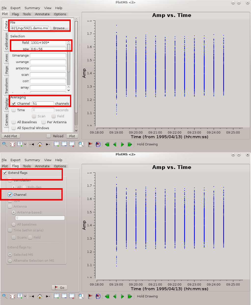
The figure at right highlights the settings needed for effective editing of a spectral line data set. The key settings are as follows.
- Specify the measurement set in File Location; the Browse button allows you to hunt down the measurement set.
- It's better to edit one source at a time. In the illustrated example, the flux / bandpass calibrator 1331+305* is displayed.
- Specify channel averaging. At the time of this writing casaplotms was not particularly versatile at specifying channel ranges, and so for now the specification is just an average over all channels. Ultimately you should be able to target specific ranges of channels.
- Ideally you want the channels to have the same (u, v) coverage (projected baseline spacings as viewed from the source); otherwise, the beam (point spread function) will be different for each channel. Therefore, if you flag data from a given channel it's usually a good idea to flag those data from all channels. Under the Flagging tab, specify Extend flags to Channel.
With these settings, interactive flagging proceeds as for continuum data. When you're satisfied with the edits, File → Quit to return to the CASA prompt.
Appendix: Python Notes
os.environ.get
It's worth having a look at the output of the os.environ.get command to understand the python syntax (alternative: os.getenv). You can think of os.environ as a list of operating system environment variables, and get is a method that extracts information about the requested environment variable, here, CASAPATH. Get returns a string of whitespace separated information, and .split() turns that string into a list. The array index [0] extracts the first element of that list, which contains the path.
To illustrate, here is some example python I/O in CASA.
CASA <12>: print os.environ.get('CASAPATH')
/usr/lib64/casapy/30.0.9709test-001 linux local el5bld64b

CASA <13>: print os.environ.get('CASAPATH').split()
['/usr/lib64/casapy/30.0.9709test-001', 'linux', 'local', 'el5bld64b']

CASA <14>: print os.environ.get('CASAPATH').split()[0]
/usr/lib64/casapy/30.0.9709test-001