Sunspot Band6 Imaging for CASA 6.6.1

Last checked on CASA Version 6.5.4

Overview

This guide features CARTA, the “Cube Analysis and Rendering Tool for Astronomy,” which is the new NRAO visualization tool for images and cubes. The CASA viewer (imview) has not been maintained for a few years and will be removed from future versions of CASA. We strongly recommend using CARTA, as it provides a much more efficient, stable, and feature rich user experience. A comparison of the CASA viewer and CARTA, as well as instructions on how to use CARTA at NRAO, is provided in the CARTA section of the CASA docs.

This portion of the guide will cover the image synthesis of a sunspot. It begins where Sunspot_Band6_Calibration_for_CASA_6.5.4 is completed. If you completed the calibration, you may continue working in the directory Sunspot_Band6_UncalibratedData.

If you did not complete the calibration portion of the guide, the calibrated visibility data is available to download at Sunspot_Band6#Obtaining the Data. Once the download has finished, unpack and cd to the directory:

# In bash
tar -xvzf Sunspot_Band6_CalibratedData.tgz
cd Sunspot_Band6_CalibratedData

Confirm your version of CASA

This guide has been written for CASA release 6.5. Please confirm your version before proceeding.

# In CASA
from casatools import version
vernum = str(version()[0])+'.'+str(version()[1])
print("You are using CASA ver. "+vernum)
if float(vernum) < 6.5:
 print("YOUR VERSION OF CASA IS TOO OLD FOR THIS GUIDE.")
 print("PLEASE UPDATE IT BEFORE PROCEEDING.")
else:
 print("Your version of CASA is appropriate for this guide.")

Flag the surplus subscans and baselines

Fig. 1. The plot of the FieldID of the Sun scans as a function of the time.

Define our ASDM and split, calibrated MS name.

# In CASA
asdm = 'uid___A002_Xae00c5_X2a8d'
msc = asdm + '.ms.split.cal'

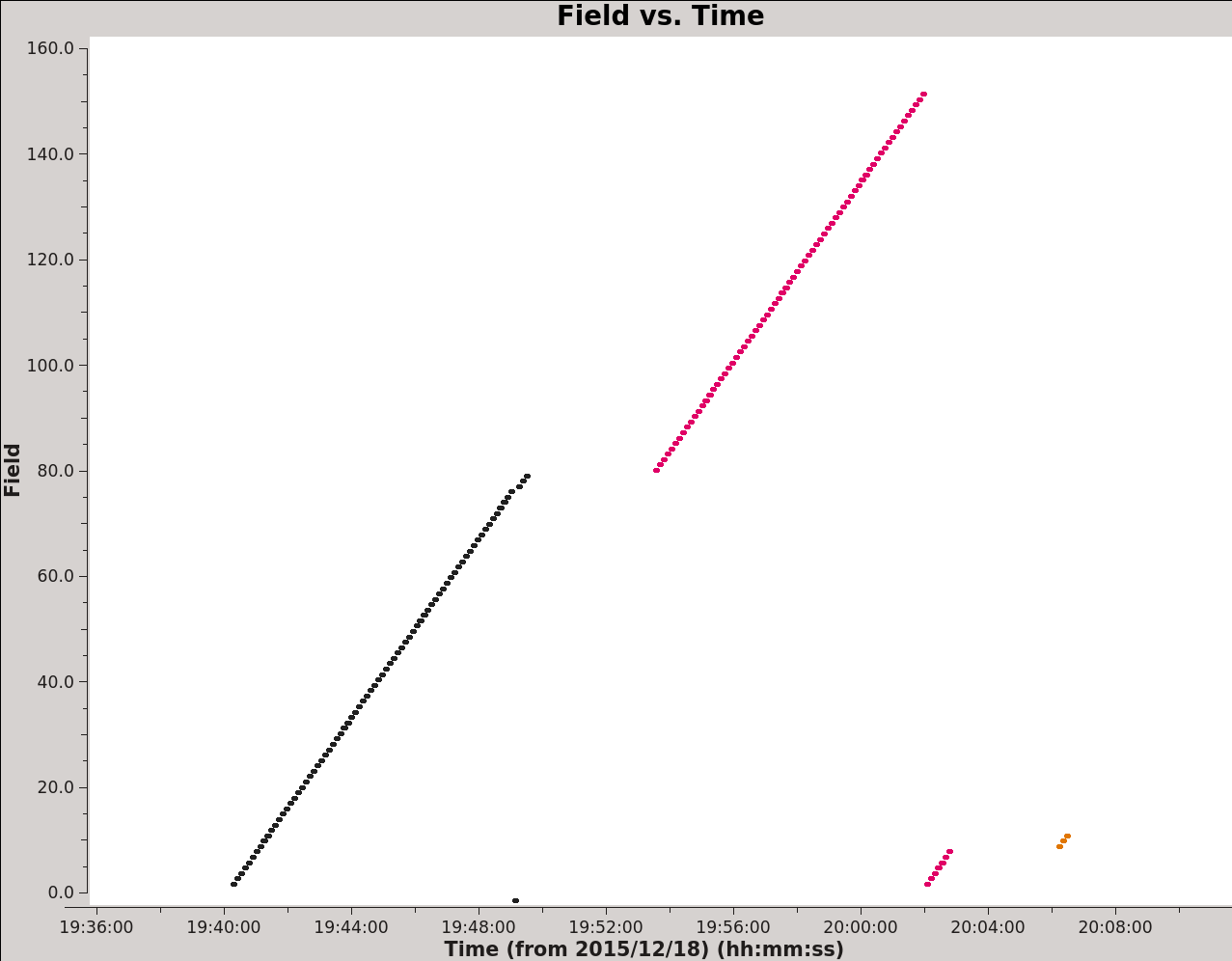
The actual duration of the observation does not exactly equal the required duration of the 149-pointing mosaic. Hence, some fields of the mosaic were observed twice, as shown in Figure 1 made with plotms.

# In CASA
plotms(vis=msc, field='0,3~150', xaxis='time', yaxis='field', coloraxis='scan', plotfile='field_vs_time.png', overwrite=True)

Although the visibility data of the surplus scans are valid, it is better that they are not used for the image synthesis, considering the uniformity of the sensitivity. For this reason, we flag the surplus scans with flagdata.

# In CASA
flagdata(vis=msc, mode='manual', timerange='2015/12/18/20:02:35~20:08:20', flagbackup=False)

The center of the 12m-array is about 200m distant from the center of the 7m-array. See Sunspot_Band6_Calibration_for_CASA_6.5.4#Antenna_List. The 12m-7m baselines have a negative impact on image synthesis (artificial stripes appear) when observations are performed with a compact 12m-array (C-1, 2). On the other hand, 12m-7m baselines can be useful for science when a larger configuration is used (C-3, 4), which includes many >200m baselines between 12m antennas. Therefore, it is necessary to consider the antenna configuration for flagging 12m-7m baseline data. In our case, we flag these baselines.

# In CASA
flagdata(vis=msc, mode='manual', antenna='CM*&DV*;CM*&DA*', flagbackup=False)

Continuum imaging

Now we are ready to synthesize a sunspot image from the visibilities. For the image synthesis, we execute the following tclean command.

Fig. 2. The cleaned continuum image, the residual map, and the primary beam cutoff at 0.73 (note the color scale).

# In CASA
import os
os.system('rm -rf AR12470_B6AllSpw_I.*')

tclean(
vis=msc,
field='0,3~150',
spw='0,1,2,3',
imagename='AR12470_B6AllSpw_I',
imsize=[512, 512],
cell='0.4 arcsec',
phasecenter=0,
stokes='I',
specmode='mfs',
interactive=False,
usemask='pb',
pbmask=0.73,
pblimit=0.73,
gridder='mosaic',
mosweight=True,
deconvolver='clark',
pbcor=False,
weighting='briggs',
robust=1.0,
niter=100000,
gain=0.1,
threshold='1.0Jy'
)

Fig. 3. The pattern of mosaic AFTER the re-calculation of the direction. See Sunspot_Band6_Calibration_for_CASA_6.5.4#Re-calculation_of_the_direction.

To obtain good SNR of the image, we synthesize an image from the data including all spectral windows. Here we comment on the parameters that are the special measures for our solar image synthesis.

• usemask='pb'
• pbmask=0.73
• pblimit=0.73

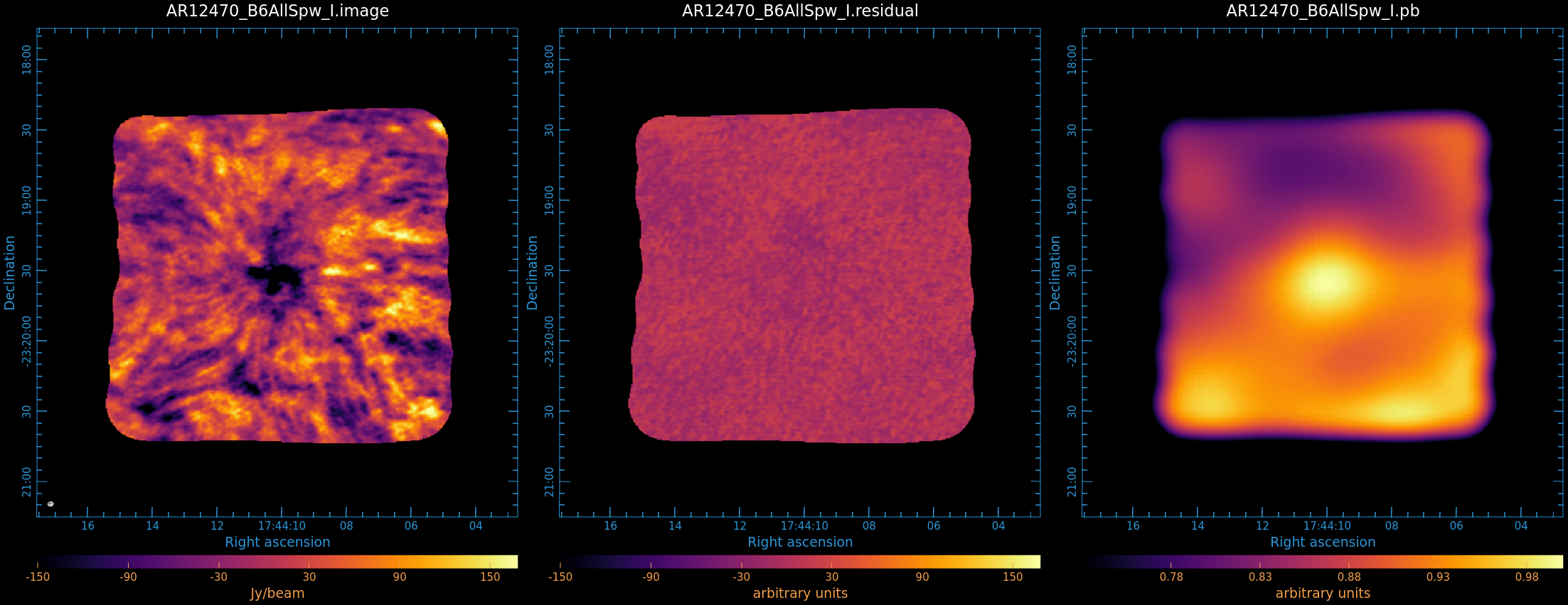
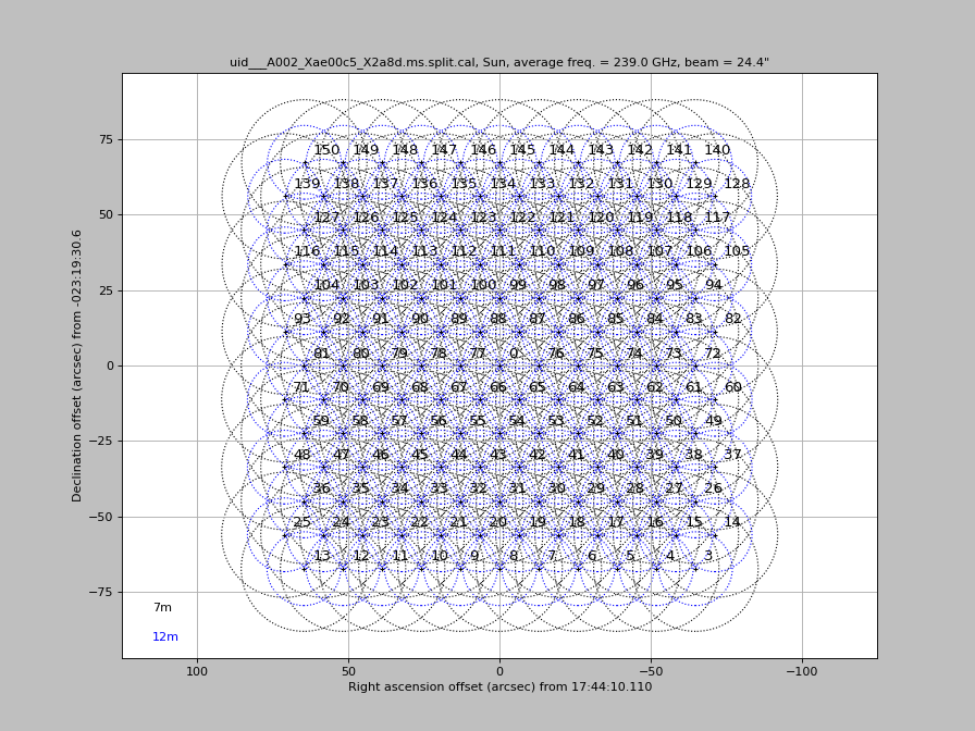
In most cases of solar observations, the field of view (FoV) of the map is filled up with solar structures. Therefore, ideally, the clean mask for the solar image synthesis is the same as the FoV. Since the observation was done with the 7m + 12m heterogeneous array, the FoV of the 7m-array is not the same as that of the 12m-array, and the area near the outer edge of the FoV is observed only with 7m-array, as shown in Figure 3. If the clean mask includes the area, the synthesized map will include remarkable artificial structures. To avoid the artificial structure, we need to make a clean mask that is smaller than the FoV of the 12m-array. In this example, the image cutoff is chosen to be the area where the effective response of the primary beam is larger than 0.73, as shown in Figure 2. We mask this entire area.

• gridder='mosaic'
• mosweight=True

To deal with the data obtained with a heterogeneous 7m+12m array, we need to set gridder='mosaic', even if we had single-pointing data. In most solar cases, the average brightness of a field might be significantly different from that of the other fields. Therefore, we use mosweight=True function. See CARMA_spectral_line_mosaic_M99_3.2#Deconvolution_and_Imaging.

• weighting='briggs'
• robust=1.0

The briggs weighting option is used for the solar image synthesis. The longest baseline of the 12m-array for the observation is shorter than that of C40-1. However, the visibility data includes >200m baselines, because the center of the 12m-array is about 200m distant from the center of the 7m-array. We have flagged these 7m-12m baselines above. The robust parameter is set to 0.5 by default. We choose robust=1.0, and which is nearer to natural weighting at +2.0 (as opposed to uniform at -2.0). Different values for robust may be chosen and compared.

After tclean has finished, you can now open the image in CARTA. If using NRAO machines, you can open a new terminal tab, cd to the working directory, then type:

# in terminal
carta --no_browser

Copy the output URL into a browser to view your CARTA session. Figure 2 shows the synthesized image, the residuals, and the primary beam displayed in CARTA. Select and load:
AR12470_B6AllSpw_I.image
AR12470_B6AllSpw_I.residual
AR12470_B6AllSpw_I.pb

Primary beam correction and creating of the FITS file

To do the primary beam correction and create the FITS file of the corrected map, we use impbcor and exportfits.

# In CASA
impbcor(imagename='AR12470_B6AllSpw_I.image', pbimage='AR12470_B6AllSpw_I.pb',
outfile='AR12470_B6AllSpw_I.pbcor', mode='divide')

exportfits(imagename='AR12470_B6AllSpw_I.pbcor', fitsimage='AR12470_B6AllSpw_I.fits')

Note: The FITS file can be imported to the data-analysis environment based on SolarSoftWare (SSW) + IDL without any modification, but the coordinate system is the RA/Dec coordinate. You have to convert from the RA/Dec coordinate system to the heliocentric coordinate system (X-cen/Y-cen) for the co-alignment with other solar instrument’s data.