VLA 5 GHz continuum survey of Seyfert galaxies 6.4.1
This particular tutorial demonstrates how to calibrate a VLA continuum survey, consisting of a flux denisty scale calibrator, target sources, and their respective complex gain calibrators. What distinguishes this example is that it includes multiple target sources and multiple complex gain calibrators.
Importing from the VLA Archive and Preliminary Data Inspection
Download your data from the VLA Archive; in this example we'll use the publicly available survey AG733, which consists of VLA C-configuration, C-band (5 GHz) continuum observations of a handful of Seyfert galaxies. It's helpful to make a directory to store the VLA archive data and the CASA measurement sets before starting CASA. We call this directory AG733 and place the downloaded file into it. Linux commands are given throughout this tutorial; it is up to you to know how to create directories, change your current working directory, and get a listing of the files in the directory if using a different operating system such as MacOS or Windows.
Doing a search for AG733 in the archive search field will return two data sets, one for December 9, 2006 and one for December 13, 2006. This tutorial will be using the December 9, 2006 data set. Click on the icon of a clipboard next to the file name to select it for download. Then click on the Download button. A pop-up will appear asking you where do you want the download to go to. Make sure that the destination directory is world readable, then click on the Submit Request button.
We will also want to check the observing log for this observation. Go to the observing log website and search on a narrow date range (the values of 2006/12/08 and 2006/12/10 were used). There will be a single entry for AG733. Click on the PDF link to download the file. Open the PDF file to review the observing log. Note that antennas 23 and 26 were being used for EVLA testing and have been excluded (flagged) from this data set.
The archive system will place the filename.exp data file, in this case AG733_1_54078.16663_54078.27045.exp, in a set of nested directories that also have the name of the data set (including the .exp extension). The directory structure is: download_job_code/AG733_1_54078.16663_54078.27045.exp/AG733_1_54078.16663_54078.27045.exp/AG733_1_54078.16663_54078.27045.exp. The download_job_code is generated by the archive, while the sub- and sub-sub directories will have the name of the data file. For ease of use you will probably want to move the filename.exp to somewhere else, such as the top level of the directory AG733 which was created earlier.
# At Linux OS level
cd AG733
# to get the most current CASA release with integrated pipeline tasks,
# as of this writing 6.4.1-12-pipeline-2022.2.0.64:
casa-pipe
# to get a listing of CASA versions available: casa -ls
# to use a version of CASA that is not the default: casa -r version_number
# for this tutorial we will be using the casa-pipe command to run CASA 6.4.1
To load the data in CASA, we employ the importvla command.
# In CASA
# Before importing, get rid of any
# original version of the measurement set
if os.path.exists('ag733.ms'): rmtables('ag733.ms')
# The following importvla command assumes that
# you are running CASA in the same directory as the data set
importvla(archivefiles=['AG733_1_54078.16663_54078.27045.exp'],vis='ag733.ms')
The output measurement set, i.e., the data to be worked on, is ag733.ms.
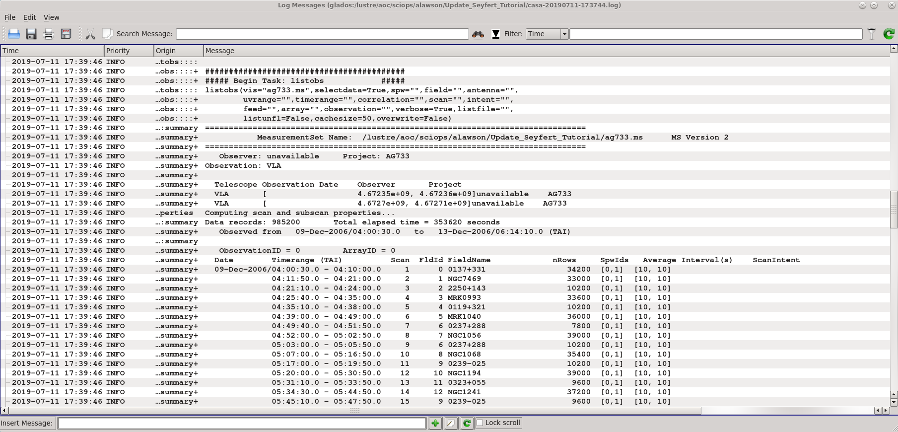
listobs provides a list of scans, sources and their respective indices, and antennas (Figure 1). If you wish to have listobs create an output text file, set the parameter listfile='output_filename.txt'

# In CASA
listobs('ag733.ms')
# for an output listing:
# listobs('ag733.ms',listfile='output_filename.txt')
# the following command will give you a pared down version of the listobs output in the CASA logger window
vishead('ag733.ms')
You can get a plot of antennas using plotants (Figure 2). The antennas plot aids the selection of a reference antenna.
# In CASA
plotants(vis='ag733.ms',figfile='ag733_plotants.png')
Use an image viewer such as xv to view the ag733_plotants.png file to find your reference antenna; the antenna VA05 looks like a reasonable choice. You may want to close plotants before moving on in the script to avoid locked tables.
Note: Some older VLA data may give errors in more recent CASA versions when attempting to generate a plot of antennas. If this occurs, use the listobs task and choose an antenna that was located on a pad close to the center of the array (Pads numbers increase with distance from the center of the array, ie. "VLA:_N1" and "EVLA:W2" are pads close to the center of the array, where as, "VLA:_N18" is not).

Also note on the plotants image that there are antennas listed as "VA" or "EA". The antennas listed as "VA" are the pre-upgrade antennas, while those listed as "EA" will be the antennas that have been upgraded. When you go to flag data, make sure that you are using the correct identifier for the antenna, e.g., "VA05" or "EA26".
Viewing and Editing the Measurement Set
This technique is detailed in the tutorial Data flagging with plotms. Here's a shorter version.
# In CASA
plotms()
plotms brings up a graphical display that allows you to plot various aspects of your data (Figure 3).
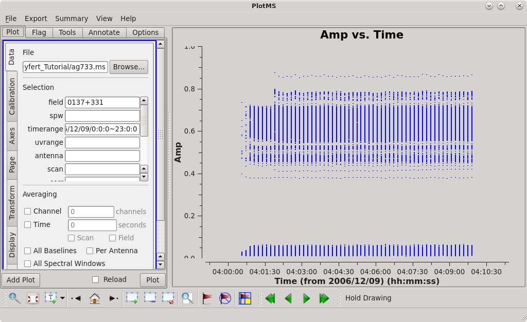
In this example, the measurement set was selected by navigating to and highlighting the measurement set ag733.ms (which will look like a directory to your file browser, because measurement sets are actually directory structures). A specific subset of data (the flux density scale calibrator 3C48 = 0137+331) was selected by specifying in the appropriate "Data -> Selection" box:
- field = 0137+331
For this specific field, we see no obvious bad data. Note that the low points are actually cross-polarization data; you can see this by entering:
- corr = RR, LL
Which will display only the RR, LL data and not the cross-polarization data (LR, RL).
If we leave the field and timerange filter boxes blank and plot, we see a number of visibilities with extremely large amplitudes. If you have trouble seeing the points, first rescale the amplitude range by going into the "Axes" tab and in the second parameters box where it has Amp, set the range from 0 to 60, click on the Reload box just left to the Plot button and replot the image. If this still isn't good enough, you can adjust the size of the points by going to "Display", setting "Unflagged Points Symbol" to "Custom", and selecting a larger pixel size for the "circle", "square", or "diamond" options and replotting. Highlight these few extremely high amplitude points and flag them as was done above. Now we'll reload the plot by selecting the "Reload" checkbox and clicking "Plot". When the plot reloads with its new adjusted scale, we notice that there are even more bad points. By highlighting and locating these new bad points (described in detail in the data flagging with plotms tutorial), we find most of the bad data can be attributed to one antenna, 'VA15', at specific times, and one time range where all antennas contribute. Close inspection will show there is also some bad data on VA05 and VA22 as well. You may need to use the Zoom Tool ![]() to see all of the bad points clearly. In the text below we flag these points using flagdata; you can also flag data interactively in the plotms display (though this is not encouraged since it does not save backup versions of the flags, and it can be easy to flag data by mistake or miss data that's not plotted).
to see all of the bad points clearly. In the text below we flag these points using flagdata; you can also flag data interactively in the plotms display (though this is not encouraged since it does not save backup versions of the flags, and it can be easy to flag data by mistake or miss data that's not plotted).
# In CASA
# flag the first 45 seconds as antennas were not all on source
flagdata(vis='ag733.ms', timerange='2006/12/09/04:00:00~04:00:45')
# a check showed that EA26 was not used during the observation, therefore it does not need to be flagged
# next flag the remaining problematic antennas and/or time range where all antennas were involved
flagdata(vis='ag733.ms', antenna='VA15', timerange='2006/12/09/04:45:10.0~04:45:20.0')
flagdata(vis='ag733.ms', antenna='VA15', timerange='2006/12/09/06:12:30.0~06:14:10.0')
flagdata(vis='ag733.ms', antenna='VA05', timerange='2006/12/09/04:30:00.0~04:30:10.0')
flagdata(vis='ag733.ms', antenna='VA22', timerange='2006/12/09/06:28:10.0~06:28:20.0')
flagdata(vis='ag733.ms', timerange='2006/12/09/06:24:50.0~06:25:00.0')
Plot the data again to make sure the amplitudes look reasonable (if plotms is already open, just hit Shift+Plot to reload with the current flags):
# In CASA
plotms()
Careful with Cross-Pols
By default, plotms plots all of the data, including cross-polarization. All those low-amplitude points in your data are probably not junk, they are real cross-polarization data. We will not be using the cross-polarization data for this tutorial, so it can be ignored. Flagging those data will cause calibration issues. Take a look at the tutorial data flagging with plotms.
When flagging data with plotms, a reminder that all data that are flagged can not be recovered as there are no backup versions. Whenever possible, it is recommended to flag with flagdata (as seen above) and keep careful track of what you flag in a separate file.
A Python Interlude
CASA uses python as an interactive wrapper and scripting language. Python offers the ability to define global variables on the fly, and it's worth using such variables to take care of bookkeeping. The setting of variables for this data set can come in handy due to the multiple science targets (seen in the example below as the variable sourcelist) and their associated complex gain calibrators (CG_callist). By setting this list up once, you can eliminate potential typographical errors in the future along with having to re-type the calibrator and source names.
First we'll define some list variables that store calibrator and source information.
# In CASA
FDS_callist = ['0137+331']
CG_callist = ['2250+143', '0119+321', '0237+288', '0239-025',
                '0323+055', '0339-017', '0423-013']
sourcelist = ['NGC7469', 'MRK0993', 'MRK1040', 'NGC1056', 'NGC1068',
              'NGC1194', 'NGC1241', 'NGC1320', 'F04385-0828',
              'NGC1667']
allcals = FDS_callist + CG_callist
print(allcals)
It will also be helpful later to have a way of referencing which complex gain calibrator should be assigned to which source. We can define the matching explicitly by using a dictionary variable.
# In CASA
calDict = {'NGC7469':'2250+143',
           'MRK0993':'0119+321',
           'MRK1040':'0237+288',
           'NGC1056':'0237+288',
           'NGC1068':'0239-025',
           'NGC1194':'0323+055',
           'NGC1241':'0323+055',
           'NGC1320':'0339-017',
           'F04385-0828':'0423-013',
           'NGC1667':'0423-013'}
Those variables being defined, we can proceed with the calibration (and not have to type source and calibrator names over and over).
Calibration
Set the Flux Denisty Scale
CASA sets the flux density scale using an observation of a flux density scale calibrator (here, 0137+331) and the task setjy. For this example, we'll determine the calibration in reference to a model image of the calibrator source. Look at the inputs of setjy by typing inp which will display the different inputs and a short description for the CASA task. For the first run of setjy we will retrieve a listing of the models available in CASA for the flux density scale calibrators.
# In CASA
# restore setjy back to its defaults
default setjy
# shows several of the current and possible input parameters for the current task
inp
vis = 'ag733.ms'
listmodel=True
go
From the list of models, we will select 3C48_C.im and tell setjy to use this model and apply it to our observation of 0137+331. We will also tell setjy to set the usescratch parameter to True so that the value is written into the MODEL column.
# In CASA
setjy(vis='ag733.ms',field='0137+331',model='3C48_C.im',usescratch=True)
setjy will return a Python dictionary to the terminal and to the logger. In the output to the display look for spectral windows 0 and 1.
{'0': {'0': {'fluxd': array([5.32591724, 0.        , 0.        , 0.        ])},
  '1': {'fluxd': array([5.37901211, 0.        , 0.        , 0.        ])},
  'fieldName': '0137+331'},
 'format': "{field Id: {spw Id: {fluxd: [I,Q,U,V] in Jy}, 'fieldName':field name }}"}
The amplitude value that setjy adjusted the flux density scale calibrator in the MODEL column is ~5.3 Jy for spw 0 and 1 (the value just after "array"). You can plot this with plotms by setting the following values:
- Data tab: field = 0, corr=RR,LL
- Axes tab: Data = Amp, Column = model
If you plot this and the amplitude is zero, rerun setjy and be sure to turn the parameter userscratch=True. Otherwise a "virtual" MODEL column will be used to calculate the fluxscale value but it will not get written to the MODEL column.
Determine calibration solutions
At this stage the data have an overall flux density scaling determined, but full gain solutions aren't there yet. The relevant task is gaincal, which will produce the table cal.G.
# In CASA
# get rid of any old versions of the calibration tables
# will give a warning if the tables don't already exist, which can be safely ignored
rmtables('cal.G')
rmtables('gc.cal')
# First we'll generate an antenna zenith-angle dependent gain curve calibration table
gencal(vis='ag733.ms', caltype='gc', caltable='gc.cal')
#
# Some caution on the following step. The solution interval is set to 'inf,' meaning to average over entire
# scans of each calibrator in turn. If a given scan is longer than the coherence time (esp. on long baselines),
# some decorrelation will occur and the flux density scale calibration will be thrown off. Suggest, e.g., solint='1min' or solint='2min'
# as reasonable alternatives to solint='inf'. Trial and error may be your friend here.
#
gaincal(vis='ag733.ms',caltable='cal.G', field=','.join(allcals), solint='inf',
        refant='VA05', gaintable=['gc.cal'], append=False)
plotms(vis='cal.G', coloraxis='Antenna1', yaxis='amp', xaxis='time', timerange='2006/12/09/04:0:0~06:30:0')
There's some python trickery buried in this example. If you are unfamiliar with the string method join, try the following example. Recall that we had defined the variable allcals above in A Python Interlude.
# In CASA
print allcals
print ','.join(allcals)
It's worth playing with the timerange, etc. in plotms to explore the solutions.
Using the task fluxscale, bootstrap the flux density scale onto the complex gain calibrators.
# In CASA
rmtables('cal.Gflx') # remove any old versions of the calibration table, if necessary
myFluxes = fluxscale(vis='ag733.ms', caltable='cal.G', reference=','.join(FDS_callist),
                     transfer=','.join(CG_callist), fluxtable='cal.Gflx', append=False)
Here, the calibration table cal.G is modified and stored as 'cal.Gflx.' The Python dictionary "myFluxes" will also contain information about the flux density scaling and other useful tidbits (type "myFluxes" to see its contents). So far, solutions have been generated only for the calibrators, and they have not yet been transfered to the sources.
We could equally well have used reference='0137+337', but use of the join method allows for the more general possibility of multiple flux density scale calibrators.
Apply the Calibrations
The task in CASA is applycal. We loop over sources and calibrators to properly match them:
# In CASA
for source, calibrator in calDict.items():
    applycal(vis='ag733.ms', field=source,
             gaintable='cal.Gflx', gainfield=calibrator)
Baseline-based corrections
Although it makes only modest improvements for the present example, observations including a mix of EVLA and VLA telescopes may benefit from performing baseline-based corrections on a strong calibrator. Now that we have initial antenna-based solutions, we can use blcal.
# In CASA
default('blcal')
vis = 'ag733.ms'
# output baseline-based calibration solutions
caltable = 'cal.BL'
# use the strong flux density scale calibrator to determine baseline-based solutions
field = '0137+331'
# generate a solution for each calibrator scan
solint = 'inf'
gaintable = 'cal.Gflx'
# calibration table with the best antenna-based solutions, so far
gainfield = '0137+331'
# calibrator for the BL calibrator; in this example, gain cal and bl cal are the same
interp = 'nearest'
# enter the time range for the data
timerange = '2006/12/09/0:0:0~24:0:0'
blcal()
This operation generates the calibration table cal.BL. Solutions can be inspected with plotms. Now we have to use applycal again to apply both the antenna-based and baseline-based calibration solutions to the data.
# In CASA
for source, calibrator in calDict.items():
    applycal(vis='ag733.ms', field=source,
             gaintable=['cal.Gflx','cal.BL'], gainfield=calibrator)
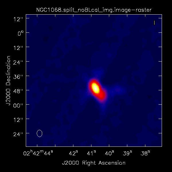
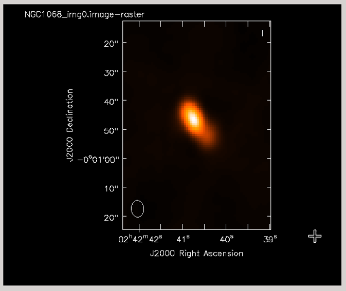
Did the blcal operation make a difference here? Getting ahead of ourselves a little, the plots at right show the initial tclean images of NGC1068, one with blcal applied, and one without, and both images are displayed with the same stretch (Figures 4A, 4B). There does appear a slight reduction of artifacts with blcal applied, but of course your mileage will vary.
Splitting the calibrated source data from the multisource measurement set
To split the calibrated source data out of the measurement set, use the CASA task split.
# In CASA
splitfile = 'NGC1667.split.ms'
rmtables(splitfile) # get rid of any old versions before splitting
split(vis='ag733.ms',outputvis=splitfile, datacolumn='corrected', field='NGC1667')
Instead of having to manually repeat the split task for each source, you can take advantage of scripting to loop over the sources:
# In CASA
for source in sourcelist:
    splitfile = source + '.split.ms'
    rmtables(splitfile)
    split(vis='ag733.ms',outputvis=splitfile,
          datacolumn='corrected', field=source)
Imaging
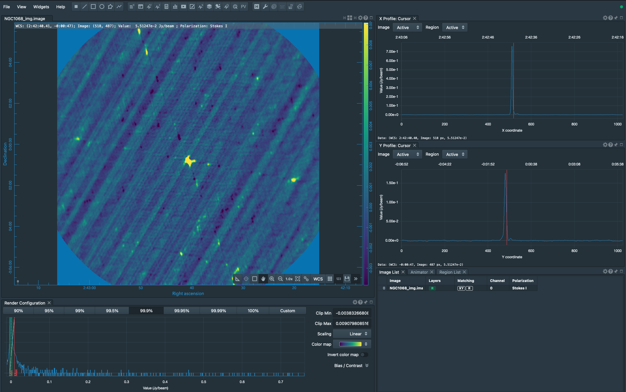
Use tclean for imaging and clean deconvolution. Like IMAGR in AIPS, it's worth some time reviewing all of the options. A list of some of the various keywords is given in the example, below. Most of the options should be relatively familiar to the AIPS user.
For this snapshot survey, the example chooses a fairly conservative slow clean to accommodate the less-than-ideal beam. You could probably get away with more efficient cleaning, but it's better to play it safe in scripted self-calibration.
# In CASA
default(tclean)
savemodel           =      'modelcolumn'
specmode            =      'mfs'
niter               =      1000
gain                =      0.1
threshold           =      '4.5e-5Jy'
deconvolver         =      'hogbom'
cyclefactor         =      3
interactive         =      False
mask                =      []
imsize              =      [1024, 1024]
cell                =      ['0.75arcsec', '0.75arcsec']
stokes              =      'I'
weighting           =      'natural'
uvtaper             =      []
pbcor               =      False
pblimit             =      0.1
selectdata          =      False
vis                 =      'NGC1068.split.ms'
imagename           =      'NGC1068_img'
rmtables(imagename + '*')
tclean()
While you can still user viewer or imview within CASA as of 6.4.1, NRAO strongly encourages that CARTA be used to view your images (Figure 5).
In the interest of time for this tutorial, we've chosen to only image NGC1068; however, should one be interested, all of the sources can be imaged by looping over a similar tclean command.
# In CASA
default(tclean)
savemodel           =      'modelcolumn'
specmode            =      'mfs'
niter               =      1000
gain                =      0.1
threshold           =      '4.5e-5Jy'
deconvolver         =      'hogbom'
cyclefactor         =      3
interactive         =      False
mask                =      []
imsize              =      [1024, 1024]
cell                =      ['0.75arcsec', '0.75arcsec']
stokes              =      'I'
weighting           =      'natural'
uvtaper             =      []
pbcor               =      False
pblimit             =      0.1
selectdata          =      False
for source in sourcelist:
    splitfile = source + '.split.ms'
    vis = splitfile
    imagename = source + '_img'
    rmtables(imagename + '*') # get ride of earlier versions of the image
    tclean()
Self-calibration
There's not much more that can be done for the fainter sources, but the brighter sources will almost certainly show some residual calibration artifacts that can be cleaned up with self-calibration. The strategy is to repeat using the primary calibration application gaincal, only this time we use the source itself as a calibrator.
NGC 1068 is a good example of a difficult source. Firstly, it's very bright, so residual complex gain calibration errors should be obvious. Secondly, like the larger fraction of the sky, it's located painfully close to the celestial equator, meaning that the (u,v) coverage is particularly poor.
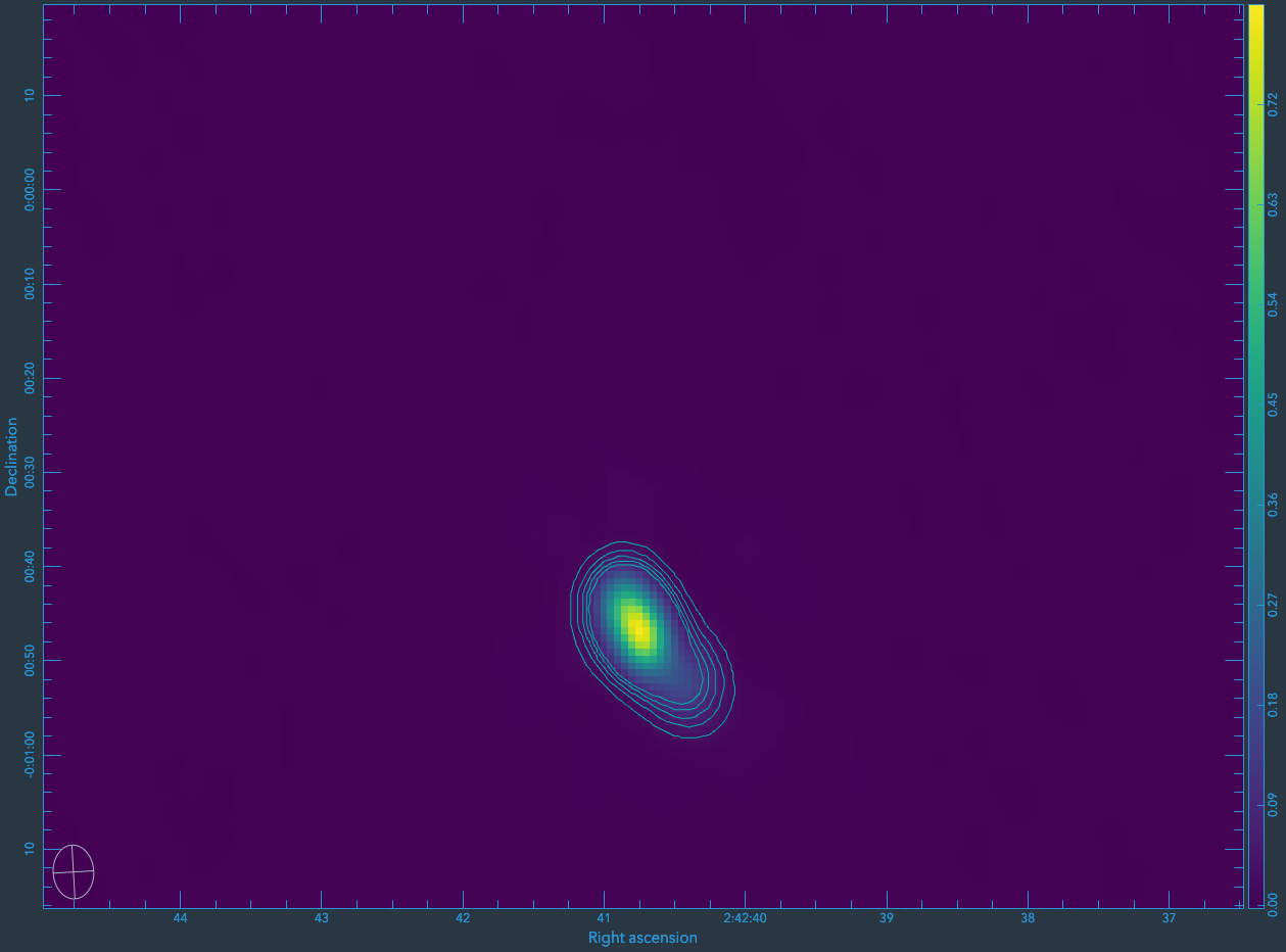
To view the calibration artifacts, use CARTA to display the image of NGC 1068, but adjust the display levels so that the displayed image saturates at 30 mJy by setting the min / max clipping range (min: -0.005, max: 0.03).
You can see some residual systematics in the background and sidelobe artifacts that suggest the complex gain calibration isn't as good as it might be.
The process of self-calibration will involve iterating between (i) improved tclean models of the source and (i+1) improved calibrations generated by gaincal. For this example, we will repeatedly generate new calibration tables so that we can avoid using accum.
Step i
In principle, we could start with the initial tclean model that we generated above. However, we'll take a more cautious approach and re-run tclean interactively.
# In CASA
source = 'NGC1068' # set up a global variable to store the source we're working on
tget tclean
vis = source + '.split.ms'
imagename = source + '_img0'
interactive = True
cycleniter = 100
go
The trick to interactive cleaning is to draw clean boxes around the sources as they appear in the residual image. By default, clean boxes are set by right-clicking on the image and dragging. The box can be edited until you double right-click inside the box, which then sets that box for cleaning. Press the green icon to continue cleaning the image; on the next major cycle, a new residual map will be displayed, affording the option to add clean boxes as new sources appear where they were once swamped by sidelobes.
Of course, for self-calibration, it pays to stop the cleaning early when artifacts start to appear in the residuals.
Step i + 1
To start, we should already have a clean model for NGC 1068 stored in the visibility database. Now we can set up gaincal.
# In CASA
default('gaincal') # reset inputs for gaincal
vis = source + '.split.ms'
caltable = source + '.gcal0'
gaintype = 'G'
calmode = 'p' # phase-only self-calibration at this stage
solint = '10 min' # set up a fairly coarse correction interval in this early stage
minsnr = 3.0
gaintable = ''
field = source
gainfield = source
gaincal() # or go
Pause for Reflection and Troubleshooting
Self-calibration is a method to fine-tune your original calibration, and, as such, should produce relatively small complex gain corrections assuming the primary calibration was applied correctly. Now is a good time to run plotms on your new calibration table (NGC1068.gcal0) to make sure the phase corrections range from a few to perhaps 10 or 20 degrees. If you see phase corrections greatly exceeding 20 degrees, then there's a chance the primary calibration wasn't applied to the split database correctly (you could check this by searching your CASA Log file for errors during the applycal tasks). To check the phase corrections, run the following and step through each antenna:
# In CASA
plotms(caltable, iteraxis='antenna', xaxis='time', yaxis='phase', plotrange=[-1,-1,-180,180])
# If you want a more detailed view of the phases:
plotms(caltable, iteraxis='antenna', xaxis='time', yaxis='phase', plotrange=[-1,-1,-20,20])
Step i + 2
Assuming plotms gave reasonable results, next apply the calibration.
# In CASA
default('applycal')
vis = source + '.split.ms'
gaintable = source + '.gcal0'
gainfield = source
go
And now we can generate a new tclean model.
# In CASA
tget tclean
imagename=source + '_img1' # choose an image root name that matches the future cal table to facilitate bookkeeping
go
Further Steps
Assuming things are going well, we can now continue to repeat the process until we are satisfied with the image.
# In CASA
tget gaincal
caltable = source +'.gcal1'
solint = '5 min' # halve the solution interval.
go

# good idea to plotms() again

tget applycal
gaintable = source + '.gcal1'
go

tget tclean
imagename = source + '_img2'
go
And so on, decreasing the solution interval as much as the S/N and sampling allow.
Note that gaincal always uses the 'data' column (not the recently self-calibrated 'corrected' column) to find gain solutions. Therefore, these iterations simply serve to improve the data model, and gain solutions at each iteration are independent (e.g., the solution from the second self calibration iteration does not accumulate on top of the solution from the first interval. Use the CASA task accum if you wish to accumulate gain solutions).
One Last Iteration: Amplitude & Phase Self Calibration
After you have improved the phase calibration as much as possible, one last iteration where both phase and amplitude are calibrated can be beneficial. A&P self calibration should be performed with long solution intervals---typically the length of a scan.
# In CASA
default('gaincal') # reset inputs for gaincal
vis = source + '.split.ms'
caltable = source + '.gcalap'
gaintype = 'G'
calmode = 'ap' # it's finally time to calibrate amplitudes, too
solint = 'inf' # one solution interval per scan (in conjunction with combine='')
combine = ''
minsnr = 3.0
gaintable = source + '.gcal1' # apply your best phase calibration on the fly.
gaincal() # or go
Here, we are applying the best phase calibration solution on the fly by setting the gaintable parameter, so that this 'ap' self calibration iteration will only make small tweaks on top of the phase solutions we just worked so hard to find. Check your solutions in plotms---amplitudes should not vary much and should be close to unity. Complex gain tweaks should be minimal and close to zero. If the solutions look reasonable, go ahead and apply the calibration:
# In CASA
default('applycal')
vis = source + '.split.ms'
gaintable = [source + '.gcal1', source + '.gcalap']
gainfield = source
go
The critical difference here from phase-only self calibration iterations is that we are applying two gain tables---the best phase solutions (source + '.gcal1') and the A&P solutions (source + '.gcalap'). Now you should be ready for one final imaging run with tclean! For consistency, we will run it with the same command we used the first time:
# In CASA
default(tclean)
savemodel           =      'modelcolumn'
specmode            =      'mfs'
niter               =      500
gain                =      0.1
threshold           =      '4.5e-5Jy'
deconvolver         =      'hogbom'
cyclefactor         =      3
interactive         =      False
mask                =      []
imsize              =      [1024, 1024]
cell                =      ['0.75arcsec', '0.75arcsec']
stokes              =      'I'
weighting           =      'natural'
uvtaper             =      []
pbcor               =      False
pblimit             =      0.1
selectdata          =      False
vis                 =      'NGC1068.split.ms'
imagename           =      'NGC1068_img4'
rmtables(imagename + '*') # get rid of earlier versions of the image
tclean()
You can use CARTA to inspect your final image.
Last checked on CASA Version 6.4.1