EVLA spectral line IRC10216
This tutorial is under construction. There are several things still to be added
in addition to overall polish and further annotation:
* screen captures of task inputs
* more about cleaning in general
* more on image analysis
* multiscale clean maybe

For the time being (until release candidate is built) you want to run this on casapy-test
Overview
This tutorial describes the data reduction for two spectral lines observed toward the AGB star IRC+10216. This carbon star, which is a few times more massive than our sun, is nearing the end of its life and is thought to be in the process of forming a planetary nebula.
In this EVLA OSRO1 mode observation one subband was observed in each of two basebands, the subbands were centered on the HC3N and SiS lines near 36 GHz. The raw data were loaded into CASA with importevla, where zero and shadowed data were flagged. Then the data were "split", so we could average from the native 1 second integrations to 10 seconds, select only antennas with Ka-band receivers, and select only spectral windows (called spw in CASA) with Ka-band data. This produces a significantly smaller dataset for processing.
The post-split averaged data can be downloaded from http://casa.nrao.edu/Data/EVLA/IRC10216/day2_TDEM0003_10s_norx.tar
Information from observing log:
There are no Ka-band receivers on ea11, ea13, ea14, ea16, ea17, ea18, ea26
Antennas ea10, ea06 are out of the array
Antenna ea12 is newly back
The pointing is often bad on ea15
Antennas ea10, ea12, ea22 do not have good baseline positions
Initial Inspection and Flagging
# In CASA
listobs(vis='day2_TDEM0003_10s_norx')
Below we have cut and pasted the most relevant output from the logger.
Fields: 4
  ID   Code Name         RA            Decl           Epoch   SrcId nVis
  2    D    J0954+1743   09:54:56.8236 +17.43.31.2224 J2000   2     65326
  3    NONE IRC+10216    09:47:57.3820 +13.16.40.6600 J2000   3     208242
  5    F    J1229+0203   12:29:06.6997 +02.03.08.5982 J2000   5     10836
  7    E    J1331+3030   13:31:08.2880 +30.30.32.9589 J2000   7     5814
   (nVis = Total number of time/baseline visibilities per field)
Spectral Windows:  (2 unique spectral windows and 1 unique polarization setups)
  SpwID  #Chans Frame Ch1(MHz)    ChanWid(kHz)TotBW(kHz)  Ref(MHz)    Corrs
  0          64 TOPO  36387.2295  125         8000        36387.2295  RR  RL  LR  LL
  1          64 TOPO  36304.542   125         8000        36304.542   RR  RL  LR  LL
Sources: 10
  ID   Name         SpwId RestFreq(MHz)  SysVel(km/s)
  0    J1008+0730   0     0.03639232     -0.026
  0    J1008+0730   1     0.03639232     -0.026
  2    J0954+1743   0     0.03639232     -0.026
  2    J0954+1743   1     0.03639232     -0.026
  3    IRC+10216    0     0.03639232     -0.026
  3    IRC+10216    1     0.03639232     -0.026
  5    J1229+0203   0     0.03639232     -0.026
  5    J1229+0203   1     0.03639232     -0.026
  7    J1331+3030   0     0.03639232     -0.026
  7    J1331+3030   1     0.03639232     -0.026
Antennas: 19:
  ID   Name  Station   Diam.    Long.         Lat.
  0    ea01  W09       25.0 m   -107.37.25.2  +33.53.51.0
  1    ea02  E02       25.0 m   -107.37.04.4  +33.54.01.1
  2    ea03  E09       25.0 m   -107.36.45.1  +33.53.53.6
  3    ea04  W01       25.0 m   -107.37.05.9  +33.54.00.5
  4    ea05  W08       25.0 m   -107.37.21.6  +33.53.53.0
  5    ea07  N06       25.0 m   -107.37.06.9  +33.54.10.3
  6    ea08  N01       25.0 m   -107.37.06.0  +33.54.01.8
  7    ea09  E06       25.0 m   -107.36.55.6  +33.53.57.7
  8    ea12  E08       25.0 m   -107.36.48.9  +33.53.55.1
  9    ea15  W06       25.0 m   -107.37.15.6  +33.53.56.4
  10   ea19  W04       25.0 m   -107.37.10.8  +33.53.59.1
  11   ea20  N05       25.0 m   -107.37.06.7  +33.54.08.0
  12   ea21  E01       25.0 m   -107.37.05.7  +33.53.59.2
  13   ea22  N04       25.0 m   -107.37.06.5  +33.54.06.1
  14   ea23  E07       25.0 m   -107.36.52.4  +33.53.56.5
  15   ea24  W05       25.0 m   -107.37.13.0  +33.53.57.8
  16   ea25  N02       25.0 m   -107.37.06.2  +33.54.03.5
  17   ea27  E03       25.0 m   -107.37.02.8  +33.54.00.5
  18   ea28  N08       25.0 m   -107.37.07.5  +33.54.15.8
Summary of Observing Strategy
Gain Calibrator: J0954+1743 field id=2
Bandpass Calibrator: J1229+0203   field id=5
Flux Calibrator: J1331+3030 (3C286) field id=7
Target: IRC+10216  field id=3
Ka-band spws = 0,1
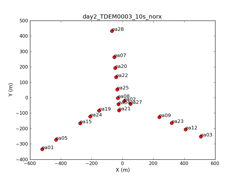
Look at a graphical plot of the antenna locations and save hardcopy in case you want it later. This will be useful for picking a reference antenna -- typically a good choice is an antenna close to the center of the array. Unless it shows problems after inspection of the data, we provisionally chose ea02.
# In CASA
plotants(vis='day2_TDEM0003_10s_norx',figfile='ant_locations.png')
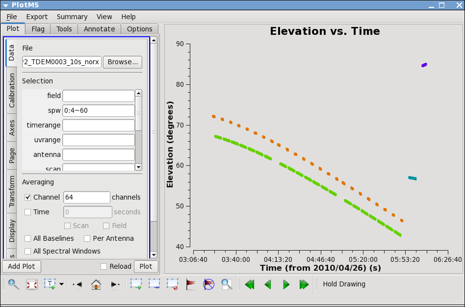
Next, let's look at the elevation as a function of time for all sources. It's not the case for these data, but if the elevation is very low (usually at start or end of track) you may want to flag. Also, how near in elevation your flux calibrator is to your target will impact your ultimate absolute flux calibration accuracy. Unfortunately, the target and flux calibrator are not particularly well-matched for this observation, as y ou can show by plotting the elevation for each source:
# In CASA
plotms(vis='day2_TDEM0003_10s_norx',
       xaxis='time',yaxis='elevation',correlation='RR,LL',
       avgchannel='64',spw='0:4~60')
Thus we are strongly dependent on the opacity and gaincurve corrections to get the flux scale right for these data. (This is something to keep in mind when planning observations!)
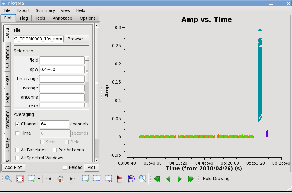
Next,let's look at all the source amplitudes as a function of time.
# In CASA
plotms(vis='day2_TDEM0003_10s_norx',
       xaxis='time',yaxis='amp',correlation='RR,LL',
       avgchannel='64',spw='0:4~60')
Select the "Display" tab and colorize by field, and click Plot button.
Now zoom in on the region very near zero amplitude for sources J0954+1743 and IRC+10216. To zoom, select the
Zoom tool in lower left corner of the plotms GUI, then you can left click to draw a box.
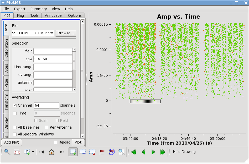
Look for the low values (you may want to zoom a few times to really see the suspect points clearly). Now use the Mark Region and Locate buttons (located along the bottom of the GUI) to see which antenna is causing problems. Since all the "located" baselines include ea12, this is the responsible antenna.
IMPORTANT NOTES ON PLOTMS:

* When using the locate button it is important to have only selected a modest number
of points with the mark region tool (see example of marked region in the thumnail),
otherwise the response will be very slow and possibly hang the tool
(all of the information will be output to your terminal window, not the logger).

* Throughout the tutorial, when you are done marking/locate use the Clear Regions
tool to get rid of the marked box before plotting other things.

* After flagdata command flagging, you have to force a complete reload of the cache
to look at the same plot again with the new flags applied. To do this change anything
in the plotms GUI (the colorize parameter, antenna, spw, anything) and hit the
plot button.

* If the plotms tool does get hung during a plot try clicking the cancel button on the
load progress GUI, and/or if you see a "table locked" message try typing
clearstat on the CASA command line.

* Occasionally plotms will get into a strange state that you cannot clear from inside.
We are working on these issues, but for now, when all else fails, exit from casapy and
restart.
Now click the unmark region button, and then go back to the zoom button to zoom in further to note exactly what the time range is: 03:41:00~04:10:00.
Check the other sideband by changing spw to 1:4~60. You will have to rezoom. If you have trouble, click on the Mark icon and then back to zoom. In spw=1, ea07 is bad from the beginning until after next pointing run: 03:21:40~04:10:00. To see this, compare the amplitudes when antenna is set to 'ea07' and when it is set to one of the other antennas, such as 'ea08'.
If you set antenna to 'ea12' and zoom in on this intial timerange, you can also see that ea12 is bad during the same time range as for spw 0. You can also see this by entering '!ea07' for antenna, which removes ea07 from the plot (in CASA selection, ! deselects).
We can set up a flagging command to get both bad antennas for the appropriate time and spw:
# In CASA
flagdata(vis='day2_TDEM0003_10s_norx',
         field=['2,3','2,3'],
         spw=['','1'],
         antenna=['ea12','ea07'],
         timerange=['03:41:00~04:10:00','03:21:40~04:10:00'])
Note that because the chosen timerange is limited to fields 2 and 3,the field parameter is not really needed; however, flagdata will run fastest if you put as many constraints as possible.
Now remove the !ea07 from antenna and replot both spw, zooming in to be sure that all obviously low points are gone. Also zoom in and check 3C286 (J1229+0203 is already obvious because it is so bright!).
Lets look more closely at IRC+10216:
# In CASA
plotms(vis='day2_TDEM0003_10s_norx',field='3',
       xaxis='time',yaxis='amp',correlation='RR,LL',
       avgchannel='64',spw='0~1:4~60')
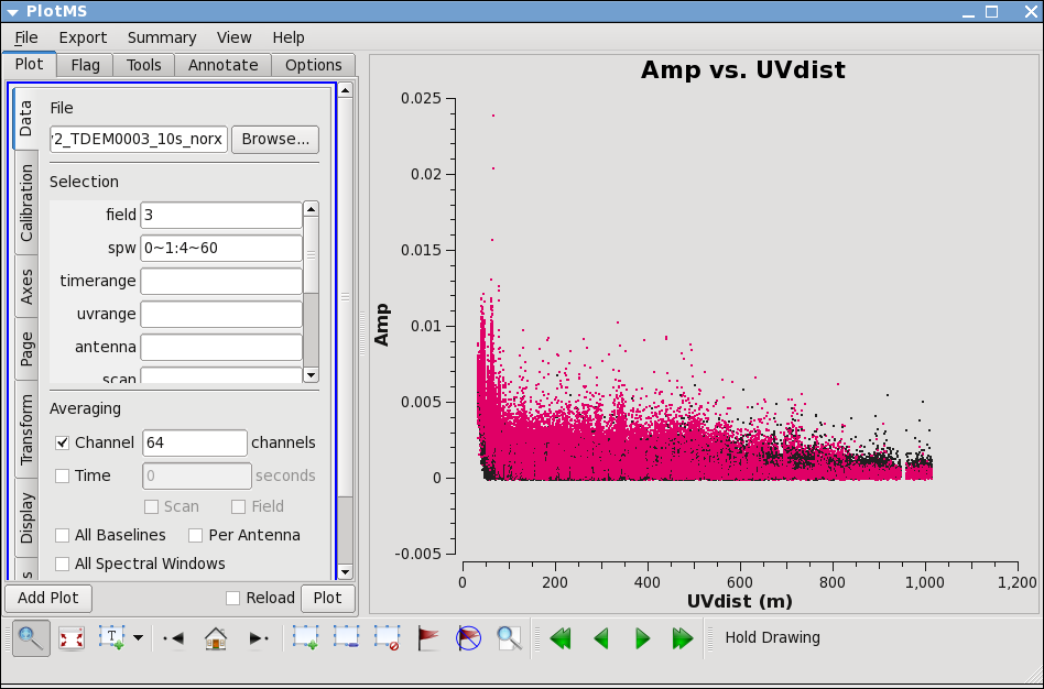
Go to the "display" tab and choose colorize by spw. You can see a that there are some noisy high points. But now try
# In CASA
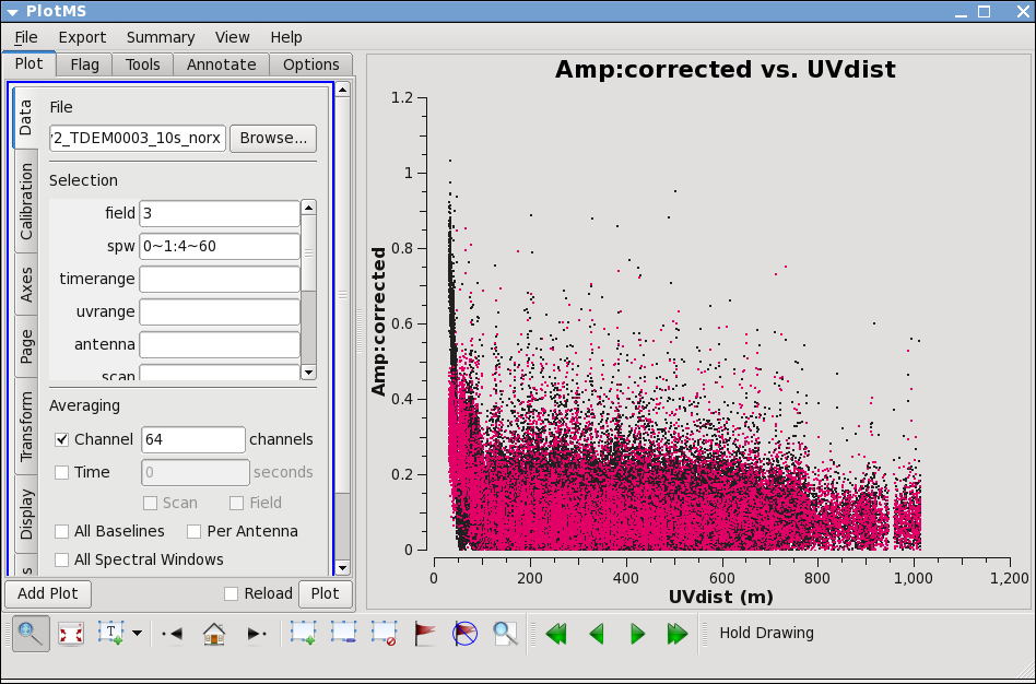
plotms(vis='day2_TDEM0003_10s_norx',field='3',
       xaxis='uvdist',yaxis='amp',correlation='RR,LL',
       avgchannel='64',spw='0~1:4~60')
Most of the high points on IRC+10216 are due to large scale emission on short baselines, but there is still some noisy stuff -- for a target like this with extended emission its best to wait until later to decide what to do about it. We will not be able to get adequate calibration for antennas that are truly bad (even if they don't stand out here) so these will be obvious later.
Set the Flux Calibrator
Next, we tell CASA to look up the appropriate fluxes for 3C286:
# In CASA
setjy(vis='day2_TDEM0003_10s_norx',field='7',spw='0~1',
      modimage='/usr/lib64/casapy/data/nrao/VLA/CalModels/3C286_K.im')
The logger output for each spw is:
setjy	  J1331+3030  spwid=  0  [I=1.692, Q=0, U=0, V=0] Jy, (Perley-Taylor 99)
setjy	  J1331+3030  spwid=  1  [I=1.695, Q=0, U=0, V=0] Jy, (Perley-Taylor 99)
The modimage location is appropriate for running CASA at the AOC. If you are running elsewhere (laptop or Mac), in a terminal type
# in a terminal, outside of CASA:
locate 3C286_K.im
to find where the models live (the models are always shipped with CASA).
Bandpass
Before determining the bandpass solution, we need to inspect phase and amplitude variations with time and frequency on the bandpass calibrator to decide how best to proceed. We limit the number of antennas to make the plot easier to see. We chose ea02 as it seems like a good candidate for the reference antenna.
# In CASA
plotms(vis='day2_TDEM0003_10s_norx',field='5',
       xaxis='channel',yaxis='phase',correlation='RR',
       avgtime='1e8',spw='0:4~60',antenna='ea02&ea23')
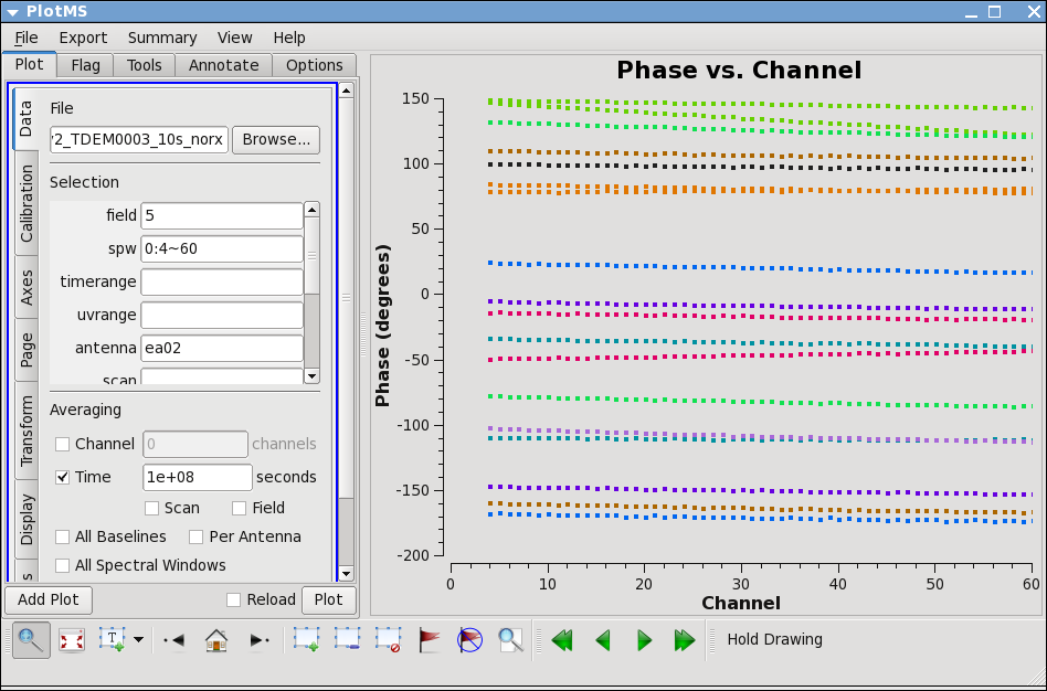
The phase variation is modest ~10 degrees. Now expand to all antennas with ea02 and select colorize by Antenna2, then hit the "Plot" button.
# In CASA
plotms(vis='day2_TDEM0003_10s_norx',field='5',
       xaxis='channel',yaxis='phase',correlation='RR',
       avgtime='1e8',spw='0:4~60',antenna='ea02')
Go to the "display" tab and chose colorize by antenna2. From this you can see that the phase variation across the bandpass is modest. Next check LL, and spw=1, both correlations. Also check other antennas if you like.
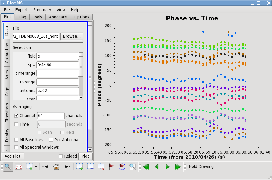
Now look at the phase as a function of time.
# In CASA
plotms(vis='day2_TDEM0003_10s_norx',field='5',
       xaxis='time',yaxis='phase',correlation='RR',
       avgchannel='64',spw='0:4~60',antenna='ea02&ea23')
Expand to all antennas with ea02
# In CASA
plotms(vis='day2_TDEM0003_10s_norx',field='5',
       xaxis='time',yaxis='phase',correlation='RR',
       avgchannel='64',spw='0:4~60',antenna='ea02')
You can see that the phase variations are smooth, but do vary significantly over the 5 minutes of observation -- in most cases by a few 10s of degrees. Zoom in to see this better if you want.
The conclusion from this investigation is that you need to correct the phase variations with time before solving for the bandpass to prevent decorrelation of the vector averaged bandpass solution. Since the phase variation as a function of channel is modest, you can average over several channels to increase the signal to noise of the phase vs. time solution. If the phase variation as a function of channel is larger you may need to use only a few channels to prevent introducing delay-based closure errors as can happen from averaging over non-bandpass corrected channels with large phase variations.
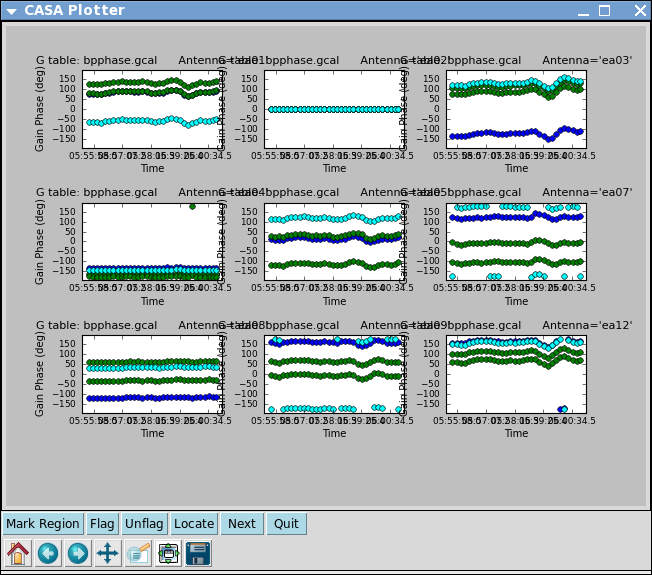
Since the bandpass calibrator is quite strong we do the phase-only
solution on the integration time of 10 seconds (solint='int').
# In CASA
gaincal(vis='day2_TDEM0003_10s_norx',caltable='bpphase.gcal',
        field='5',spw='0~1:20~40',
        refant='ea02',calmode='p',solint='int',minsnr=2.0,
        opacity=0.03,gaincurve=T)
Plot the solutions
# In CASA
plotcal(caltable='bpphase.gcal',xaxis='time',yaxis='phase',
        iteration='antenna',subplot=331,plotrange=[0,0,-180,180])
After the first set of plots appear, push the "Next" button on the GUI to see the next set of antennas.
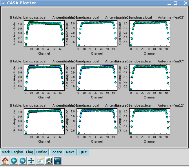
Next we can apply this phase solution on the fly while determining the bandpass solutions on the timescale of the bandpass calibrator scan (solint='inf').
# In CASA
bandpass(vis='day2_TDEM0003_10s_norx',caltable='bandpass.bcal',field='5',
        refant='ea02',solint='inf',solnorm=T,
        gaintable=['bpphase.gcal'],spwmap=[[]],
        opacity=0.03,gaincurve=T)
A few words about solint and combine:
The use of solint='inf' in bandpass will derive one bandpass solution for the whole J1229+0203 scan. Note that if there had been two observations of the bandpass calibrator (for example), this command would have combined the data from both scans to form one bandpass solution, because the default of the combine parameter for bandpass is combine='scan'. To solve for one bandpass for each bandpass calibrator scan you would also need to include combine=' ' in the bandpass call. In all calibration tasks, regardless of solint, scan boundaries are only crossed when combine='scan'. Likewise, field (spw) boundaries are only crossed if combine='field' (combine='spw'), the latter two are not generally good ideas for bandpass solutions.
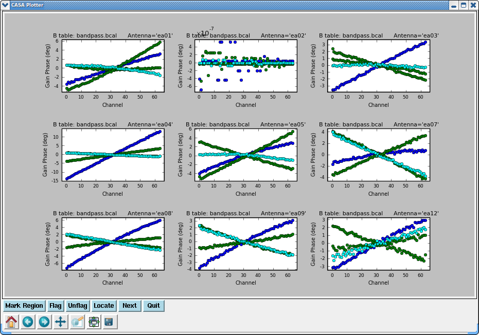
Plot the solutions, amplitude and phase:
# In CASA
plotcal(caltable='bandpass.bcal',xaxis='chan',yaxis='amp',
        iteration='antenna',subplot=331)
# In CASA
plotcal(caltable='bandpass.bcal',xaxis='chan',yaxis='phase',
        iteration='antenna',subplot=331)
Note that phases on ea12 look noiser than on other antennas. This jitter could indicate bad pointing; note that ea12 had just come back in the array.
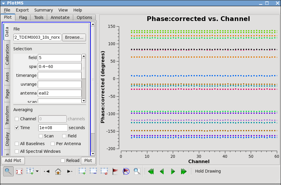
This step isn't necessary from a calibration perspective, but if you want to go ahead and check the bandpass calibration on the bandpass calibrator you can run applycal here. In future we hope to plot corrected data on-the-fly without this applycal step. Later applycals will overwrite this one, so no need to worry.
applycal(vis='day2_TDEM0003_10s_norx',field='5',
        gaintable=['bandpass.bcal'],
        spwmap=[[]],gainfield=['5'],
        opacity=0.03,gaincurve=T)
plotms(vis='day2_TDEM0003_10s_norx',field='5',
       xaxis='channel',yaxis='phase',ydatacolumn='corrected',
       correlation='RR',
       avgtime='1e8',spw='0:4~60',antenna='ea02')
plotms(vis='day2_TDEM0003_10s_norx',field='5',
       xaxis='channel',yaxis='amp',ydatacolumn='corrected',
       correlation='RR',
       avgtime='1e8',spw='0:4~60',antenna='ea02')
Note that the phase and amplitude as a function of channel are very flat now.
Gain Calibration
Now that we have a bandpass solution to apply we can solve for the antenna-based phase and amplitude gain calibration. Since the phase changes on a much shorter timescale than the amplitude, we will solve for them separately. In particular, if the phase changes significantly over a scan time, the amplitude would be decorrelated, if the un-corrected phase were averaged over this timescale. Note that we re-solve for the gain solutions of the bandpass calibrator, so we can derive new solutions that are corrected for the bandpass shape. Since the bandpass calibrator will not be used again, this is not strictly necessary, but is useful to check its calibrated flux density for example.
# In CASA
gaincal(vis='day2_TDEM0003_10s_norx',caltable='intphase.gcal',
        field='2,5,7',spw='0~1:4~60',
        refant='ea02',calmode='p',solint='int',minsnr=2.0,
        gaintable=['bandpass.bcal'],spwmap=[[]],
        opacity=0.03,gaincurve=T)
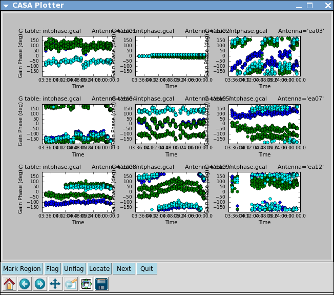
Here solint='int' coupled with calmode='p' will derive a single phase solution for each 10 second integration. Note that the bandpass table is applied on-the-fly before solving for the phase solutions, however the bandpass is NOT applied to the data permanently until applycal is run later on.
Now look at the phase solution, and note the obvious scatter within a scan time.
# In CASA
plotcal(caltable='intphase.gcal',xaxis='time',yaxis='phase',
        iteration='antenna',subplot=331,plotrange=[0,0,-180,180])
Although solint='int' (i.e. the integration time of 10 seconds) is the best choice to apply before for solving for the amplitude solutions, it is not a good idea to use this to apply to the target. This is because the phase-scatter within a scan can dominate the interpolation between calibrator scans. Instead, we also solve for the phase on the scan time, solint='inf' (but combine=' ', since we want one solution per scan) for application to the target later on. Unlike the bandpass task, for gaincal, the default of the combine parameter is combine=' '.
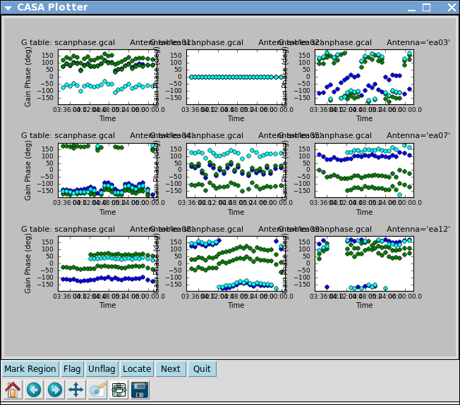
# In CASA
gaincal(vis='day2_TDEM0003_10s_norx',caltable='scanphase.gcal',
        field='2,5,7',spw='0~1:4~60',
        refant='ea02',calmode='p',solint='inf',minsnr=2.0,
        gaintable=['bandpass.bcal'],spwmap=[[]],
        opacity=0.03,gaincurve=T)
# In CASA
plotcal(caltable='scanphase.gcal',xaxis='time',yaxis='phase',
        iteration='antenna',subplot=331,plotrange=[0,0,-180,180])
Alternatively, one can also run smoothcal to smooth the solutions derived on the integration time.
Next we apply the bandpass and solint='int' phase-only calibration solutions on-the-fly to derive amplitude solutions. Here the use of solint='inf', but combine=' ' will result in one solution per scan interval.
# In CASA
gaincal(vis='day2_TDEM0003_10s_norx',caltable='amp.gcal',
        field='2,5,7',spw='0~1:4~60',
        refant='ea02',calmode='ap',solint='inf',minsnr=2.0,
        gaintable=['bandpass.bcal','intphase.gcal'],spwmap=[[],[]],
        opacity=0.03,gaincurve=T)
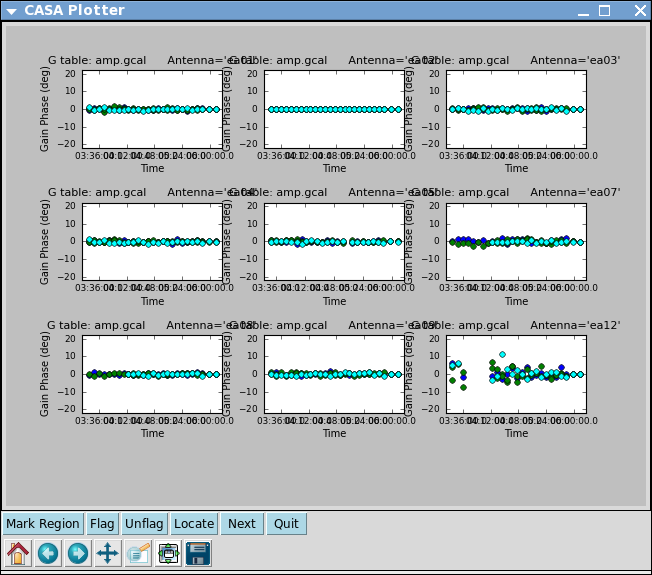
Now let's look at the resulting phase solutions. Since we have taken out the phase as best we can by applying the solint='int' phase-only solution, this plot will give a good idea of the residual phase error. If you see scatter of more than a few degrees here, you should consider going back and looking for more data to flag, particularly bad timeranges etc.
# In CASA
plotcal(caltable='amp.gcal',xaxis='time',yaxis='phase',
        iteration='antenna',subplot=331)
Indeed, both antenna ea12 (all times) and ea23 (first 1/3 of observation) show particularly large residual phase noise.
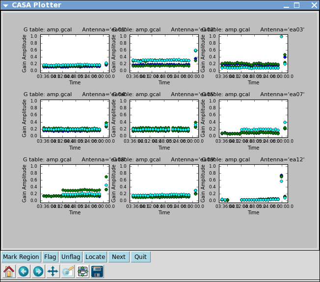
# In CASA
plotcal(caltable='amp.gcal',xaxis='time',yaxis='amp',
        iteration='antenna',subplot=331)
Note that the amplitude solutions for ea12 are very low; this is another indication that this antenna is dubious.
Next we use the flux calibrator (whose flux density was set in setjy above) to derive the flux of the other calibrators. Note that the flux table REPLACES the amp.gcal in terms of future application of the calibration to the data, i.e. the flux table contains both the amp.gcal and flux scaling. Unlike the gain calibration steps, this is not an incremental table.
# In CASA
fluxscale(vis='day2_TDEM0003_10s_norx',caltable='amp.gcal',
          fluxtable='flux.cal',reference='7')
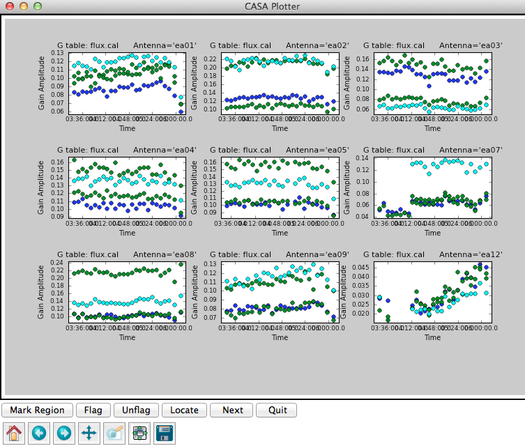
It is a good idea to note down for your records the derived flux densities:
Flux density for J0954+1743 in SpW=0# is: 0.267699 +/- 0.00103786
   (SNR = 257.934, nAnt= 19)
Flux density for J0954+1743 in SpW=1# is: 0.279468 +/- 0.000735923
   (SNR = 379.752, nAnt= 19)
Flux density for J1229+0203 in SpW=0# is: 30.5454 +/- 0
   (SNR = inf, nAnt= 19)
Flux density for J1229+0203 in SpW=1# is: 30.2306 +/- 0
   (SNR = inf, nAnt= 19)
Obviously, the signal-to-noise for J1229+0203 can't be infinity! This is just an indication that their is only one scan for this source, and we derived a scan based amplitude solution, so there is no variation to calculate.
Next, check that the flux.cal table looks as expected.
# In CASA
plotcal(caltable='flux.cal',xaxis='time',yaxis='amp',
        iteration='antenna',subplot=331)
Applycal and Inspect
Now we apply the calibration to each source, according to which tables are appropriate, and which source should be used to do that particular calibration. For the calibrators, all bandpass solutions come from the bandpass calibrator (id=5), and the phase and amplitude calibration comes from their own solutions.
# In CASA
applycal(vis='day2_TDEM0003_10s_norx',field='2',
        gaintable=['bandpass.bcal','intphase.gcal','flux.cal'],
        spwmap=[[],[],[]],gainfield=['5','2','2'],
        opacity=0.03,gaincurve=T)
# In CASA
applycal(vis='day2_TDEM0003_10s_norx',field='5',
        gaintable=['bandpass.bcal','intphase.gcal','flux.cal'],
        spwmap=[[],[],[]],gainfield=['5','5','5'],
        opacity=0.03,gaincurve=T)
# In CASA
applycal(vis='day2_TDEM0003_10s_norx',field='7',
        gaintable=['bandpass.bcal','intphase.gcal','flux.cal'],
        spwmap=[[],[],[]],gainfield=['5','7','7'],
        opacity=0.03,gaincurve=T)
For the target we apply the bandpass from id=5, and the calibration from the gain calibrator (id=2):
# In CASA
applycal(vis='day2_TDEM0003_10s_norx',field='3',
        gaintable=['bandpass.bcal','scanphase.gcal','flux.cal'],
        spwmap=[[],[],[]],gainfield=['5','2','2'],
        opacity=0.03,gaincurve=T)
Now inspect the corrected data:
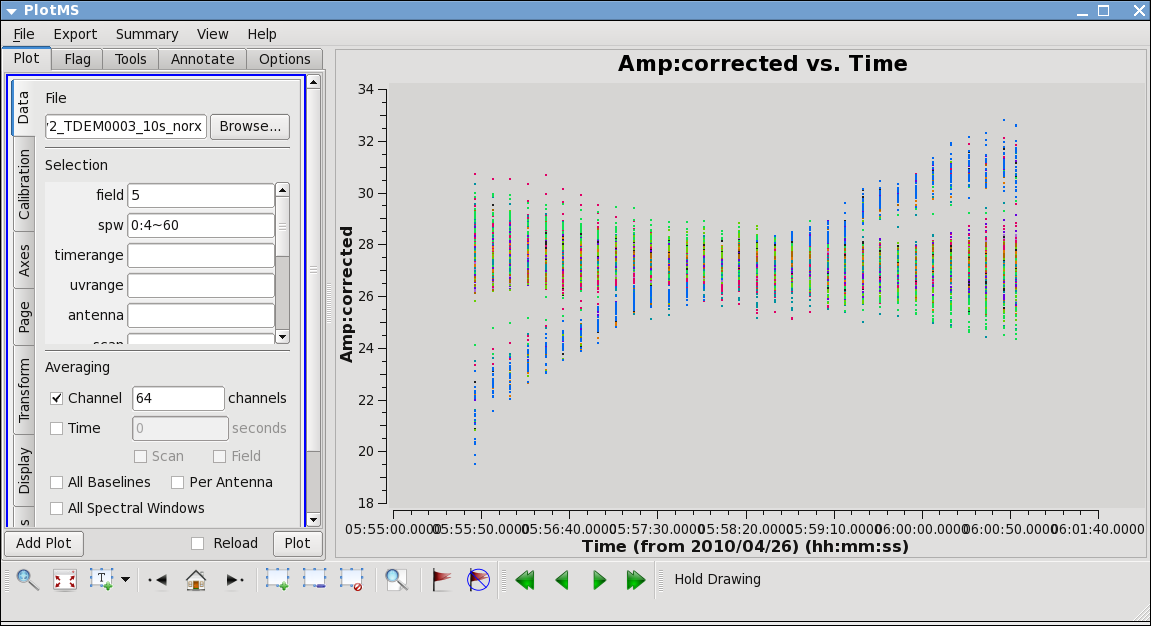
# In CASA
plotms(vis='day2_TDEM0003_10s_norx',field='5',ydatacolumn='corrected',
       xaxis='time',yaxis='amp',correlation='RR,LL',
       avgchannel='64',spw='0:4~60',antenna='')
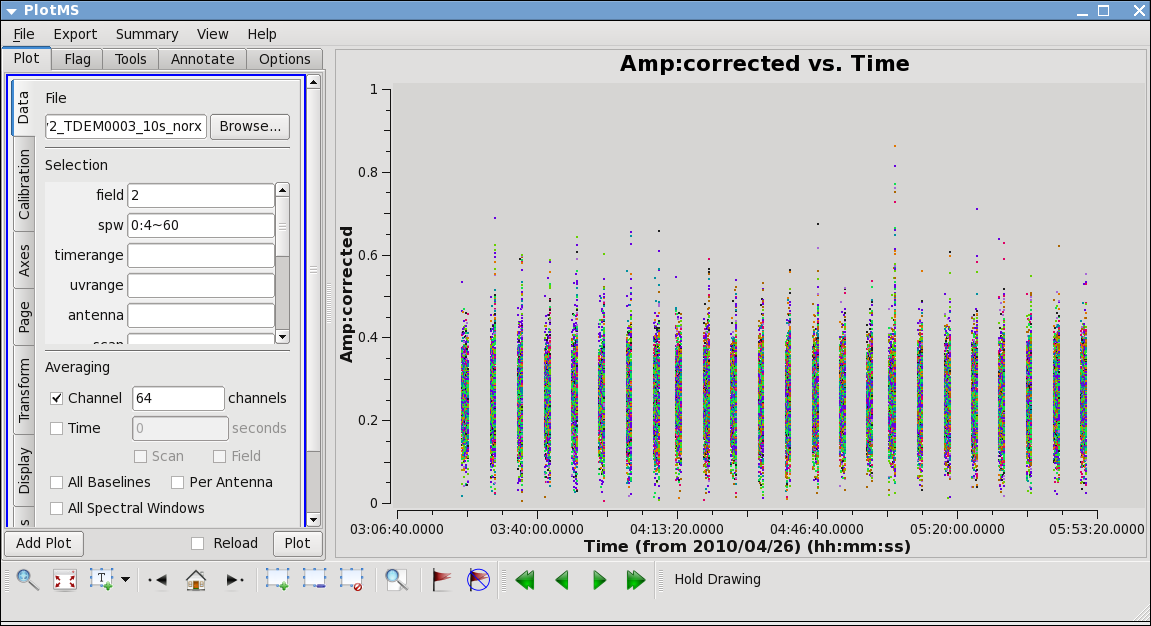
This plot shows some data deviating from the average amplitudes. Use methods described above to mark a region for a small number of deviant data points, and click "Locate". You will find that ea12 is responsible.
# In CASA
plotms(vis='day2_TDEM0003_10s_norx',field='2',ydatacolumn='corrected',
       xaxis='time',yaxis='amp',correlation='RR,LL',
       avgchannel='64',spw='0:4~60',antenna='')
Here we see some problems, with high points. Mark some regions and locate in plotms to find out which antennas and in which spws. Pay special attention to antennas that have been called out already as showing some dubious behavior.
What you find is that ea07 which we flagged spw=1 above, is also bad for the same timerange in spw=0. This was not obvious in the raw data, because spw=0 was adjusted in the on-line system by a gain attenuator, while spw=1 wasn't. So a lack of power on this antenna can look like very low (and obvious) amplitudes in spw=1 but not for spw=0. Looking carefully you'll see that ea07 is actually pretty noisy throughout.
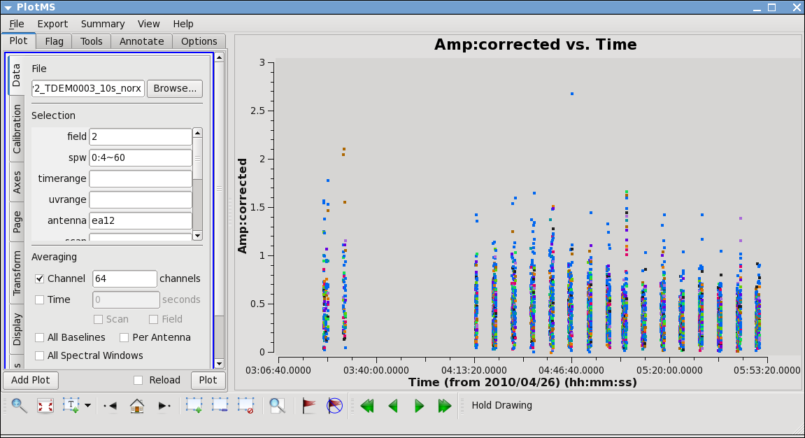
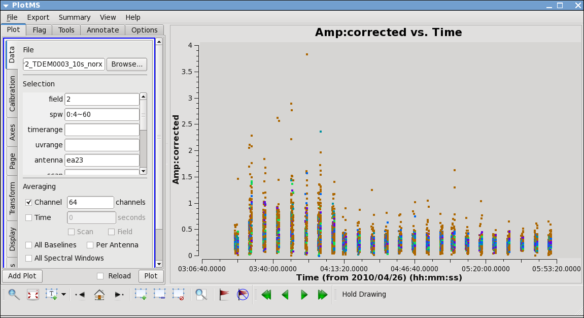
From the locate we also find that ea12 and ea23 show some high points; to see this, replot baselines using each of them alone:
plotms(vis='day2_TDEM0003_10s_norx',field='2',ydatacolumn='corrected',
       xaxis='time',yaxis='amp',correlation='RR,LL',
       avgchannel='64',spw='0:4~60',antenna='ea12')
plotms(vis='day2_TDEM0003_10s_norx',field='2',ydatacolumn='corrected',
       xaxis='time',yaxis='amp',correlation='RR,LL',
       avgchannel='64',spw='0:4~60',antenna='ea23')
ea12 needs to be flagged completely its just a bit noisy all around and ea23 is pretty noisy during the first scans between initial and second pointing. Recall that these are antennas we became suspicious of while inspecting the calibration solutions.
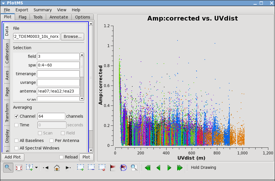
Now lets see how the target looks. Because the target has resolved structure, its best to look at it as a function of uvdistance. We'll go ahead and exclude the three antennas we already know have problems.
# In CASA
plotms(vis='day2_TDEM0003_10s_norx',field='3',ydatacolumn='corrected',
       xaxis='uvdist',yaxis='amp',correlation='RR,LL',
       avgchannel='64',spw='0:4~60',antenna='!ea07;!ea12;!ea23')
in "display" tab choose colorize by antenna2; then you can see that the spikes are caused by a single antenna. Use, zoom, mark, and locate to see which one. Also look at spw=1.
Turns out to be ea28; to confirm, replot with antenna=!ea28, and
# In CASA
plotms(vis='day2_TDEM0003_10s_norx',field='3',ydatacolumn='corrected',
       xaxis='uvdist',yaxis='amp',correlation='RR,LL',
       avgchannel='64',spw='0:4~60',antenna='!ea07;!ea12;!ea23;!ea28')
To see if it's restricted to a certain time
# In CASA
plotms(vis='day2_TDEM0003_10s_norx',field='3',ydatacolumn='corrected',
       xaxis='time',yaxis='amp',correlation='RR,LL',
       avgchannel='64',spw='0:4~60',antenna='ea28')
Baselines with ea28 clearly show issues until about two-thirds of the way through the observation.
Plot another distant antenna to compare. We will go ahead and flag it all, since its hanging far out on the north
arm by itself.
The additional data we've identified as bad need to be flagged, and then all the calibration steps will need to be run again.
# In CASA
flagdata(vis='day2_TDEM0003_10s_norx',
         field=['',''],
         spw=['',''],
         antenna=['ea07,ea12,ea28','ea07,ea23'],
         timerange=['','03:21:40~04:10:00'])
Redo Calibration after more Flagging
After flagging, you'll need to repeat the calibration steps above. Here, we append _redo to the table names to distinguish them from the first round, in case we want to compare with previous versions.
# In CASA
gaincal(vis='day2_TDEM0003_10s_norx',caltable='bpphase_redo.gcal',
        field='5',spw='0~1:20~40',
        refant='ea02',calmode='p',solint='int',minsnr=2.0,
        opacity=0.03,gaincurve=T)
# In CASA
bandpass(vis='day2_TDEM0003_10s_norx',caltable='bandpass_redo.bcal',
        field='5',
        refant='ea02',solint='inf',solnorm=T,
        gaintable=['bpphase_redo.gcal'],spwmap=[[]],
        opacity=0.03,gaincurve=T)
# In CASA
gaincal(vis='day2_TDEM0003_10s_norx',caltable='intphase_redo.gcal',
        field='2,5,7',spw='0~1:4~60',
        refant='ea02',calmode='p',solint='int',minsnr=2.0,
        gaintable=['bandpass_redo.bcal'],spwmap=[[]],
        opacity=0.03,gaincurve=T)
# In CASA
gaincal(vis='day2_TDEM0003_10s_norx',caltable='scanphase_redo.gcal',
        field='2,5,7',spw='0~1:4~60',
        refant='ea02',calmode='p',solint='inf',minsnr=2.0,
        gaintable=['bandpass_redo.bcal'],spwmap=[[]],
        opacity=0.03,gaincurve=T)
# In CASA
gaincal(vis='day2_TDEM0003_10s_norx',caltable='amp_redo.gcal',
        field='2,5,7',spw='0~1:4~60',
        refant='ea02',calmode='ap',solint='inf',minsnr=2.0,
        gaintable=['bandpass_redo.bcal','intphase_redo.gcal'],
        spwmap=[[],[]],
        opacity=0.03,gaincurve=T)
# In CASA
fluxscale(vis='day2_TDEM0003_10s_norx',caltable='amp_redo.gcal',
          fluxtable='flux_redo.cal',reference='7')
Flux density for J0954+1743 in SpW=0 is: 0.279304 +/- 0.00114727 (SNR = 243.452, nAnt= 16)
Flux density for J0954+1743 in SpW=1 is: 0.287039 +/- 0.00107576 (SNR = 266.824, nAnt= 16)
Flux density for J1229+0203 in SpW=0 is: 30.5932 +/- 0 (SNR = inf, nAnt= 16)
Flux density for J1229+0203 in SpW=1 is: 30.2475 +/- 0 (SNR = inf, nAnt= 16)
Feel free to pause here and remake the calibration solution plots from above, just be sure to put in the revised table names.
Redo Applycal and Inspect
Now, apply all the new calibrations, which will overwrite the old ones. These commands are identical to those above, with the exception of the _redo part of each calibration filename.
# In CASA
applycal(vis='day2_TDEM0003_10s_norx',field='2',
        gaintable=['bandpass_redo.bcal','intphase_redo.gcal','flux_redo.cal'],
        spwmap=[[],[],[]],gainfield=['5','2','2'],
        opacity=0.03,gaincurve=T)
# In CASA
applycal(vis='day2_TDEM0003_10s_norx',field='5',
        gaintable=['bandpass_redo.bcal','intphase_redo.gcal','flux_redo.cal'],
        spwmap=[[],[],[]],gainfield=['5','5','5'],
        opacity=0.03,gaincurve=T)
# In CASA
applycal(vis='day2_TDEM0003_10s_norx',field='7',
        gaintable=['bandpass_redo.bcal','intphase_redo.gcal','flux_redo.cal'],
        spwmap=[[],[],[]],gainfield=['5','7','7'],
        opacity=0.03,gaincurve=T)
# In CASA
applycal(vis='day2_TDEM0003_10s_norx',field='3',
        gaintable=['bandpass_redo.bcal','scanphase_redo.gcal','flux_redo.cal'],
        spwmap=[[],[],[]],gainfield=['5','2','2'],
        opacity=0.03,gaincurve=T)
Now you can inspect the calibrated data again. Except for random scatter things look pretty good.
# In CASA
plotms(vis='day2_TDEM0003_10s_norx',field='2',ydatacolumn='corrected',
       xaxis='time',yaxis='amp',correlation='RR,LL',
       avgchannel='64',spw='0:4~60',antenna='')
Lets check the target again, looking at both spws, and selecting "Display" colorize by spw. You can use the Mark and Locate buttons to assess that the remaining scatter seems random, i.e. no particular antenna or time range appears to be responsible.
# In CASA
plotms(vis='day2_TDEM0003_10s_norx',field='3',ydatacolumn='corrected',
       xaxis='uvdist',yaxis='amp',correlation='RR,LL',
       avgchannel='64',spw='0~1:4~60',antenna='')
Split
Now we split the data into individual files. This is not strictly necessary, as you can select the appropriate fields in later clean stages, but it is safer in case for example you get confused with later processing and want to fall back to this point (this is especially a good idea if you plan to do continuum subtraction or self calibration later on). It also makes smaller individual files in case you want to copy to another machine or colleague.
Here, we split off the data for the phase calibrator and the target:
# In CASA
split(vis='day2_TDEM0003_10s_norx',outputvis='J0954',
      field='2')
# In CASA
split(vis='day2_TDEM0003_10s_norx',outputvis='IRC10216',
      field='3')
To reinitialize the scratch columns for use by later tasks, we need to run clearcal for both new datasets
# In CASA
clearcal(vis='J0954')
# In CASA
clearcal(vis='IRC10216')
UV Continuum Subtraction
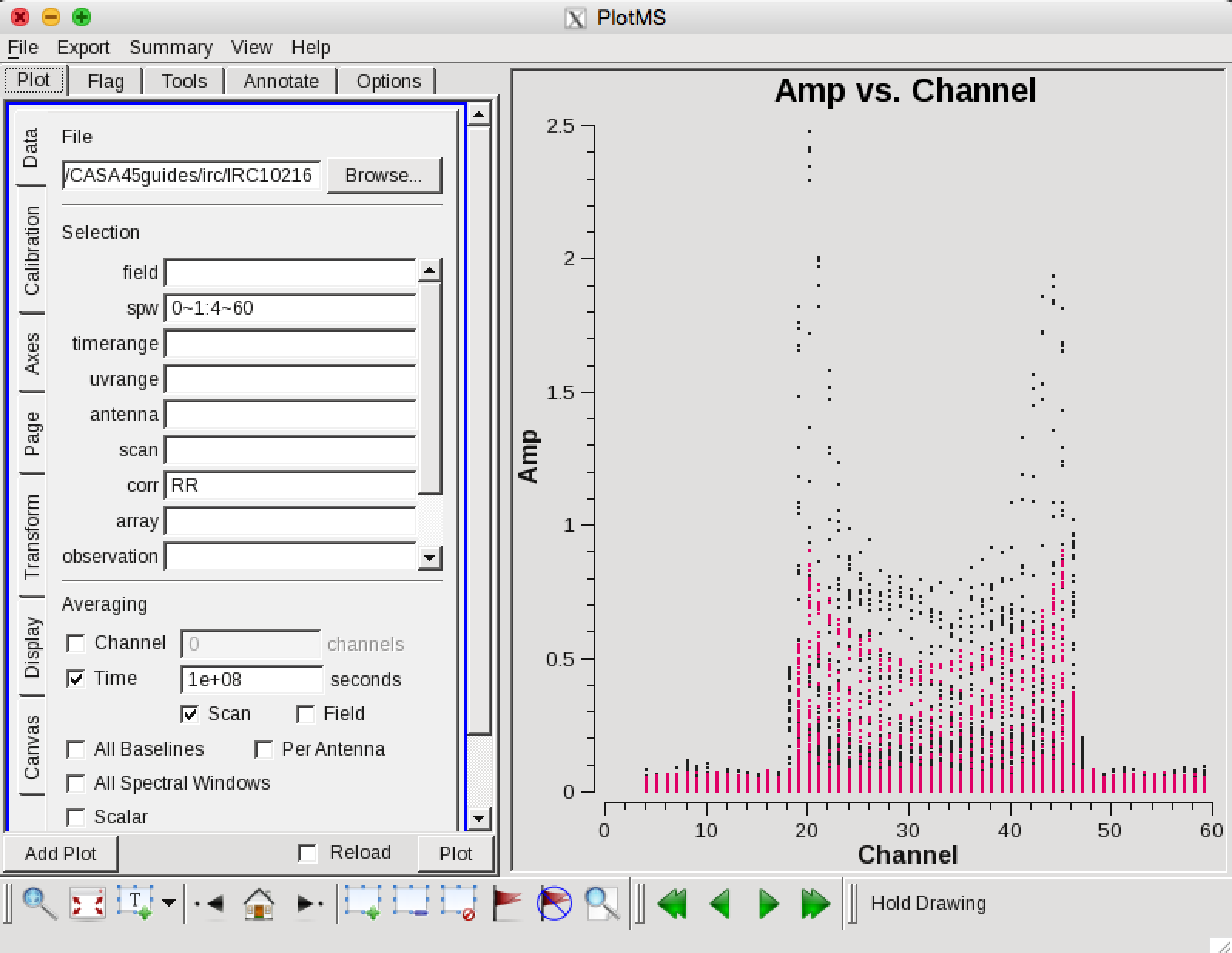
Now we can make a vector averaged uv-plot of the calibrated target spectral line data. It is important to note that you will only see signal in such a plot if (1) the data are well calibrated, (2) there is significant signal near the phase center of the observations. If this isn't true for your data, you will need to make an initial line+continuum cube to determine the line-free channels.
plotms(vis='IRC10216',field='',ydatacolumn='corrected',
       xaxis='channel',yaxis='amp',correlation='RR',
       avgtime='1e8',avgscan=T,spw='0~1:4~60',antenna='')
in the Display tab, choose colorize by spw and change the Unflagged points symbol to custom and Style of 3.
You should see the "horned profile" typical of a rotation shell. From this plot, you can guess that strong line emission is restricted to channels 18 to 47 (zoom in if necessary to see exactly what the channel numbers are).
In the Data tab you can also click on "all baselines" to average all baselines, but this is a little harder to see.
Now we want to use the line free channels to create a model of the continuum emission that can be subtracted to form a line-only dataset. We want to refrain from going to close to the edges of the band -- these channels are typically noisy, and we don't want to get too close to the line channels because we could only see strong line emission in the vector averaged uv-plot.
uvcontsub2(vis='IRC10216',fitspw='0~1:4~13;52~60',
       want_cont=T)
The "want_cont=T" will produce new two new datasets, IRC10216.contsub is the continuum subtracted line data, and IRC10216.cont is the continuum estimate (note however, that it is still a multi-channel cube).
Image the Spectral Line Data
Here we make images from the continuum-subtracted, calibrated spectral line data. Because the spectral line emission from IRC+10216 has significant extended emission, it is very important to run clean interactively, and make a clean mask.
# In CASA
clean(vis='IRC10216.contsub',imagename='IRC10216_HC3N.cube_r0.5',
      imagermode='csclean',
      imsize=300,cell=['0.4arcsec'],spw='0:5~58',
      mode='velocity',interpolation='linear',
      restfreq='36.39232GHz',outframe='LSRK',
      weighting='briggs',robust=0.5,
      interactive=T,
      threshold='3.0mJy',niter=100000)
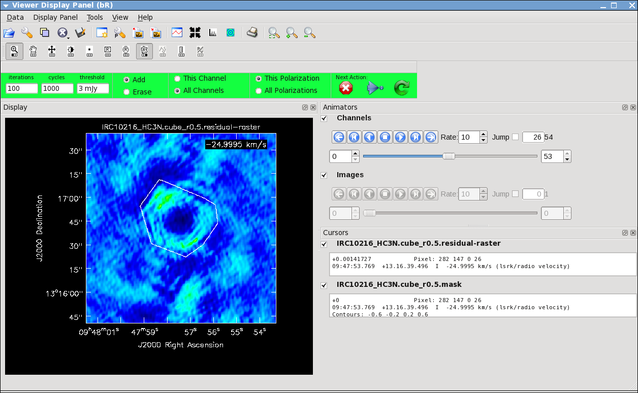
It will take a little while to grid the data, but viewer will open when it's ready to start an interactive clean. Use the "tape deck" at the bottom of the Viewer display GUI to step through to the channel with the most extended (in angular size) emission, select "all channels" for the clean mask, select the polygon tool (second in from the right) and make a single mask that applies to all channels (see example in thumbnail). Once you make the polygon region, you need to double click inside it to save the mask region -- if you see the polygon turn white you will know you succeeded. Note, that if you had the time and patience you could make a clean mask for each channel, and this would create a slightly better result.
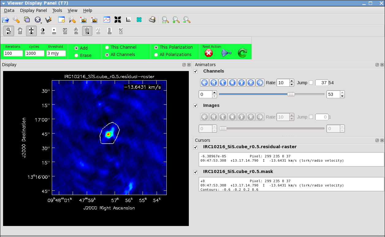
After making the mask you should check that the emission in all the other channels fits within the mask you made using the "tape deck" to move back and forth. If you need to include more area in the mask, you can chose the "erase" toggle at the top, and then encircle your existing mask with a polygon and double click inside. Then go back to "add" toggle at top and make a new mask. Alternatively, you can erase a part of the mask, or you can add to the existing mask by drawing new polygons. Feel free to experiment with this a bit.
To continue with clean use the "Next action" buttons in the green area on the Viewer Display GUI: The red X will stop clean where you are, the blue arrow will stop the interactive part of clean, but continue to clean non-interactively until reaching the stopping niter or threshold (whichever comes first), and the green arrow will clean until it reaches the "iterations" parameter on the left side of the green area.
Keep cleaning, by using the green Next Action arrow until the residual displayed in the viewer looks "noise like". To speed things up, you might change the iteration parameter in the viewer to something like 300. This parameter can also be set in the task command. You will notice that in this particular case, there are residuals that cannot be cleaned -- these are due to the extended resolved out structure on size scales larger than the array is sensitive to (the "Largest Angular Scale" or LAS that the array is sensitive to can be calculated from the shortest baseline length).
Repeat the process for the SiS line using the call below, note that the emission for this line is less extended than the HC3N -- this has to do with the different excitation requirements of the two different lines. The SiS is excited closer to the central star than the HC3N.
# In CASA
clean(vis='IRC10216.contsub',imagename='IRC10216_SiS.cube_r0.5',
      imagermode='csclean',
      imsize=300,cell=['0.4arcsec'],spw='1:5~58',
      mode='velocity',interpolation='linear',
      restfreq='36.30963GHz',outframe='LSRK',
      weighting='briggs',robust=0.5,
      interactive=T,
      threshold='3.0mJy',niter=100000)
Image the Continuum data
Below the use of mode='mfs' will make a single multi-frequency synthesis image out of the specified spw. Again you should make an interactive clean mask.
# In CASA
clean(vis='IRC10216.cont',imagename='IRC10216.36GHzcont',
      mode='mfs',imagermode='csclean',
      imsize=300,cell=['0.4arcsec'],spw='0~1:5~59',
      weighting='briggs',robust=0.5,
      interactive=T)
Image Analysis and Viewing
Next make integrated intensity maps (moment 0) and integrated velocity maps (moment 1). To do this, we'll want to know what channels the line emission starts and ends on, and also the rms noise in a single channel. So first lets open the viewer:
viewer
Then use the Viewer tape deck to see which channels have significant line emission. For HC3N, the line channel range in the cube is 11 to 40, and it is the same for SiS.
Then use the tape deck to go to a line free channel, select the box region tool and make a box. When you double click in the box, the image statistics for the whole cube will print to the terminal and for the channel you are one, it will print to a pop up window. Move the box around a bit to see what the variation is. You should get something like 2 mJy. Note that the rms is much worse in channels with strong emission because of the low dynamic range of these data. If you want the box tool to go away, hit the escape key.
Now lets make the moment 0 and moment 1 maps. For moment zero, its best to limit the calculation to image channels with significant signal in them, but not to apply a flux cutoff, as this will bias the derived integrated intensities upward.
immoments(imagename='IRC10216_HC3N.cube_r0.5.image',moments=[0],
          axis='spectral',
          chans='11~40',
          outfile='IRC10216_HC3N.cube_r0.5.image.mom0')
immoments(imagename='IRC10216_SiS.cube_r0.5.image',moments=[0],
          axis='spectral',
          chans='11~40',
          outfile='IRC10216_SiS.cube_r0.5.image.mom0')
For moment 1, it is essential to apply a conservative flux cutoff to limit the calculation to high signal-to-noise areas. Here we use about 5sigma.
immoments(imagename='IRC10216_HC3N.cube_r0.5.image/',moments=[1],
          axis='spectral',
          chans='11~40',excludepix=[-100,0.01],
          outfile='IRC10216_HC3N.cube_r0.5.image.mom1')
immoments(imagename='IRC10216_SiS.cube_r0.5.image/',moments=[1],
          axis='spectral',
          chans='11~40',excludepix=[-100,0.01],
          outfile='IRC10216_SiS.cube_r0.5.image.mom1')
Now user the viewer to further explore the images you've made.