Simulating Observations in CASA v3.0.1
As of release 3.0.0, CASA's tools to produce simulated interferometric data are quite powerful. As with all aspects of
CASA, there is a beginner-level python task interface called simdata, which calls methods in the sm C++ tool. The task interface turns a model of the sky (2 to 4 dimensions including frequency and Stokes) into the visibilities that would be measured with ALMA, (E)VLA, CARMA, SMA, ATCA, PdB, etc. The task also can produce a cleaned image of the model visibilities, compare that image with your input convolved with the synthesized beam, and calculate a fidelity image. simdata can add thermal noise (from receiver, atmosphere, and ground) to the visibilities.
The sm tool has methods that can be used to add phase delay variations, gain fluctuations and drift, cross-polarization, and (coming soon) bandpass and pointing errors to your simulated data. sm also has more flexibility in adding thermal noise than simdata, for example for new observatories that are unknown to simdata.
CASA simulation uses the aatm atmospheric model, a thin wrapper of Juan Pardo's ATM library, to accurately calculate all atmospheric corruption terms (noise, phase delay) accurately as a function of frequency and site characteristics.
Part of CASA's simulation routines are generic ephemeris and geodesy calculations available in python - see simutil.py.
simdata is under active development, documentation may lag reality, please email rindebet at nrao.edu with any questions - It's my job to help you use this software. In particular, you may find that some of the presentations and graphics below show parameter inputs that are slightly different from the latest version of CASA.
Steps to simulation
|
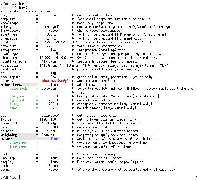
Simdata pdf presentation explaining the same things as below: File:Tutorial.dec2009.pdf 1. Install CASA simdata inputs look like this (v3.0.2; click to enlarge): the links below describe the various sections of inputs 2. Input Model - Preparing a patch of sky for simdata to pseudoobserve.
3. Antenna List - how to specify the positions and diameters of your antennas or stations. 4. Specifying Observation - how to set up what/when/how you want to observe, and the output image details 5. Corrupting Observation - (Optional) For added realism, corrupt your visibilities with thermal and phase noise. 6. Deconvolve Image (Optional) Go back from the calculated visibilities to a synthesis image |
|
Simdata2 1. Install CASA simdata2 inputs look like this (v3.0.2; click to enlarge): the links below describe the various sections of inputs 2. Input Model - Preparing a patch of sky for simdata2 to pseudoobserve.
3. Antenna List - how to specify the positions and diameters of your antennas or stations. 4. Specifying Observation - how to set up what/when/how you want to observe, and the output image details 5. Corrupting Observation - (Optional) For added realism, corrupt your visibilities with thermal and phase noise. 6. Deconvolve Image (Optional) Go back from the calculated visibilities to a synthesis image |
Technical and Planning
I always welcome input on developing the CASA simulator, and these links are meetings, technical documents, and planning discussions. Much of it won't make sense to a new user of CASA::simdata, but may be of interest to those wanting to delve deeper:
- Simulation Library This will become a library of use cases and examples illustrating different science and observation setups. It is in early stages as of Jan 2010, and we're actively seeking volunteers to turn their simulation projects into use cases.
- Jan 2010 workshop Including slides and discussion of how simdata and Simulator work "under the hood" and plans for development

