HI 21cm (1.4 GHz) spectral line data reduction: LEDA 44055
Overview
This tutorial describes the data reduction of the HI spectral line observed of the nearby (4.8 Mpc), gas-rich dwarf galaxy LEDA44055 (Figure 1: grab HST image). For its gas-rich nature, LEDA44055 is quiescent and is an Hα non-detection. Observations by the HST show a weak blue plume structure, and further inspection of GALEX archival images show some faint emission in the optical body, which taken together suggest that LEDA44055 may be in a "post-starburst" phase.
In this 1.4 GHz observation, a 16 MHz wide IF pair (A0C0 as seen in later in listobs) subband (spectral window, abbreviated as spw in CASA) using 4096 channels was observed, each channel providing ~ 1700 km/s of velocity coverage that results in a channel width of 3.906 kHz per channel. Another IF pair (B0D0) is used to acquire 1-2 GHz continuum imaging of the field; if LEDA44055 is in post-starbust phase, then it may display significant synchotron emission.
The TDEM0025 observation at the VLA was done during C-configuration and spanned 2 hours on the instrument from 31 July 2017 at 23:10 UT to 1 August 2017 at 01:10 UT. Information about the observation can be found on the corresponding VLA Observing Log and the continuation log (the observing log was split at the monthly boundary). This observing log is a record of events that transpired during the observation of the project, including weather conditions and any loss of antenna(s) and/or components that could affect the outcome of the observation.
This observation of LEDA44055 was taken as part of the Observing for University Classes program. The project code for this VLA observation is TDEM0025. This paper by Cannon et. al is the result of the observation.
How to use this CASA guide
Please use CASA 5.4.0 for this tutorial (typing casa -ls in a linux window shows the available versions and the current version; to explicitly change the current version type, e.g., casa -r 5.4.0-68)
There are at least three different ways to interact with CASA, described in more detail in Getting Started in CASA. In this guide we provide the pseudo-interactive method for every step and the interactive method for some of the steps. Since it is possible to use both methods, take care not to run the same task with identical parameters twice using both methods.
- Interactively examining task inputs. In this mode, one types taskname to load the task, inp to examine the inputs (see Figure 2), and go once those inputs have been set to your satisfaction. Allowed inputs are shown in blue and bad inputs are colored red. The input parameters themselves are changed one by one, e.g., selectdata=True. Summaries of the inputs to various tasks used in the data reduction below are provided, to illustrate which parameters need to be set. More detailed help can be obtained on any task by typing help taskname. Once a task is run, the set of inputs are stored and can be retrieved via tget taskname; subsequent runs will overwrite the previous tget file. To reset a task to its default settings type, default taskname.
# Interactive CASA
<default|tget> taskname
inp
parameter1 = value1
parameter2 = value2
(etc)
inp   (Always double check the input parameters before running the task.)
go
- Pseudo-interactively via task function calls. In this case, all of the desired inputs to a task are provided at once on the CASA command line. This tutorial is made up of such calls, which were developed by looking at the inputs for each task and deciding what needed to be changed from default values. For task function calls, only parameters that you want to be different from their defaults need to be set.
# Pseudo-interactive CASA
taskname('input parameters')
- Non-interactively via a script. A series of task function calls can be combined together into a script, and run from within CASA via execfile('scriptname.py'). This and other CASA Tutorial Guides have been designed to be extracted into a script via the script extractor by using the method described within the Extracting scripts from these tutorials page. Should you use the script generated by the script extractor for this CASA Guide, be aware that it will require some small amount of interaction related to the plotting, occasionally suggesting that you close the graphics window and hitting return in the terminal to proceed. It is in fact unnecessary to close the graphics windows (it is suggested that you do so purely to keep your desktop uncluttered).
Step 1: Obtain the Dataset
From the NRAO Data Archive enter TDEM0025 in the Project Code field and select the data set TDEM0025.sb34039638.eb34043648.57965.965492013886. (This should be the only dataset for the project). The dataset on the archive is around 85 GB in size.
You will download the dataset as an SDM file, either as a .tar file or as an uncompressed file. Under the Jansky VLA datasets options, check the "SDM-BDF dataset (all files)" button and, if you want the dataset downloaded as a .tar file, check the "Create tar file" box.
Once you have your dataset, copy it into a directory where you can launch CASA to begin the data reduction steps below. If you downloaded the dataset as a .tar file, you need to perform the following extra step to extract the dataset before beginning the data reduction steps.
#In a terminal outside of CASA:
tar -xf TDEM0025.sb34039638.eb34043648.57965.965492013886.tar
Step 2: Import the Dataset into CASA
In earlier versions of CASA, you would import your data using the CASA command importevla. With CASA 5.4.0 and higher this task has been deprecated and, while it is still functional, there will be no further support for this task and you should instead use the CASA task importasdm to import your dataset into CASA. In order to make importasdm duplicate the task importevla, several parameters will need to be set from their default values.
# Interactive CASA
default importasdm
inp
asdm='TDEM0025.sb34039638.eb34043648.57965.965492013886'
vis='TDEM0025.ms'
ocorr_mode='co'
savecmds=True
outfile='TDEM0025_onlineflags.txt'
applyflags=True
inp
go
# Psuedo-interactive CASA
importasdm(asdm='TDEM0025.sb34039638.eb34043648.57965.965492013886',vis='TDEM0025.ms',ocorr_mode='co',savecmds=True,outfile='TDEM0025_onlineflags.txt',applyflags=True)
Where:
    inp                    # lists the inputs available for this task
    adsm='SDM-BDF File ID' # this is the filename of the SDM-BDF to use
    vis='filename.ms'      # this is the name of the output measurement set created (.ms)
    ocorr_mode='co'        # the VLA is a cross-correlator
    savecmds=True          # write the online flagging commands to an output file
    outfile='filename.txt' # name of the file containing the online flags
    applyflags=True        # apply the online flags during creation of the MS
    go                     # executes the task with the given inputs
Next we will use flagcmd to look at the table of online flags. This plot will show a graphical view of the online flags, which are antenna and/or time based flags.
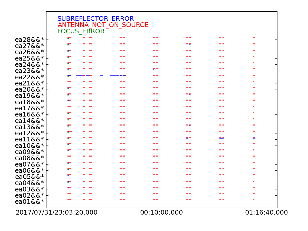
From this plot (see Figure 1), we can see that ea22 has a subreflector error during the beginning of the observation. We will flag this in a later step.
# Interactive CASA
default flagcmd
vis='TDEM0025.ms'
inpmode='table'
useapplied=True
action='plot'
savepars=True
plotfile='flagcmd-table.png'
inp
go
flagcmd(vis='TDEM0025.ms', inpmode='table', useapplied=True, action='plot', savepars=True, plotfile='flagcmd-table.png')
Step 3: Inspecting the Observation Info
Listobs
The next step is to inspect the contents of the MS using listobs. The task listobs provides almost all relevant observational parameters such as correlator setup (frequencies, bandwidths, channel number and widths, polarization products), sources, scans, scan intents, and antenna locations. Setting verbose=True will display all of the contents of the raw data and setting listfile='listobs.txt' will create a text file you can refer to later.
# Interactive CASA
default listobs
inp
vis='TDEM0025.ms'
verbose=True
listfile='listobs.txt'
inp
go
# Psuedo-interactive CASA
listobs(vis='TDEM0025.ms', verbose=True, listfile='listobs.txt')
Below is a copy/paste of a portion of the listobs output:
   Observer: Dr. John M. Cannon     Project: uid://evla/pdb/34039543
Observation: EVLA
Data records: 7480512       Total elapsed time = 7176 seconds
   Observed from   31-Jul-2017/23:10:27.0   to   01-Aug-2017/01:10:03.0 (UTC)

   ObservationID = 0         ArrayID = 0
  Date        Timerange (UTC)          Scan  FldId FieldName             nRows     SpwIds   Average Interval(s)    ScanIntent
  31-Jul-2017/23:10:27.0 - 23:11:24.0     1      0 1331+305=3C286           60021  [0,1,2,3,4,5,6,7,8]  [3, 3, 3, 3, 3, 3, 3, 3, 3] [SYSTEM_CONFIGURATION#UNSPECIFIED]
              23:11:27.0 - 23:15:54.0     2      0 1331+305=3C286          281151  [0,1,2,3,4,5,6,7,8]  [3, 3, 3, 3, 3, 3, 3, 3, 3] [CALIBRATE_BANDPASS#UNSPECIFIED,CALIBRATE_FLUX#UNSPECIFIED]
              23:15:57.0 - 23:20:21.0     3      0 1331+305=3C286          277992  [0,1,2,3,4,5,6,7,8]  [3, 3, 3, 3, 3, 3, 3, 3, 3] [CALIBRATE_BANDPASS#UNSPECIFIED,CALIBRATE_FLUX#UNSPECIFIED]
              23:20:24.0 - 23:22:21.0     4      1 J1330+2509              123201  [0,1,2,3,4,5,6,7,8]  [3, 3, 3, 3, 3, 3, 3, 3, 3] [CALIBRATE_AMPLI#UNSPECIFIED,CALIBRATE_PHASE#UNSPECIFIED]
              23:22:24.0 - 23:24:21.0     5      1 J1330+2509              123201  [0,1,2,3,4,5,6,7,8]  [3, 3, 3, 3, 3, 3, 3, 3, 3] [CALIBRATE_AMPLI#UNSPECIFIED,CALIBRATE_PHASE#UNSPECIFIED]
              23:24:24.0 - 23:30:45.0     6      2 LEDA44055               401193  [0,1,2,3,4,5,6,7,8]  [3, 3, 3, 3, 3, 3, 3, 3, 3] [OBSERVE_TARGET#UNSPECIFIED]
              23:30:48.0 - 23:37:09.0     7      2 LEDA44055               401193  [0,1,2,3,4,5,6,7,8]  [3, 3, 3, 3, 3, 3, 3, 3, 3] [OBSERVE_TARGET#UNSPECIFIED]
              23:37:12.0 - 23:43:30.0     8      2 LEDA44055               398034  [0,1,2,3,4,5,6,7,8]  [3, 3, 3, 3, 3, 3, 3, 3, 3] [OBSERVE_TARGET#UNSPECIFIED]
              23:43:33.0 - 23:45:30.0     9      1 J1330+2509              123201  [0,1,2,3,4,5,6,7,8]  [3, 3, 3, 3, 3, 3, 3, 3, 3] [CALIBRATE_AMPLI#UNSPECIFIED,CALIBRATE_PHASE#UNSPECIFIED]
              23:45:33.0 - 23:51:54.0    10      2 LEDA44055               401193  [0,1,2,3,4,5,6,7,8]  [3, 3, 3, 3, 3, 3, 3, 3, 3] [OBSERVE_TARGET#UNSPECIFIED]
              23:51:57.0 - 23:58:15.0    11      2 LEDA44055               398034  [0,1,2,3,4,5,6,7,8]  [3, 3, 3, 3, 3, 3, 3, 3, 3] [OBSERVE_TARGET#UNSPECIFIED]
              23:58:18.0 - 00:04:39.0    12      2 LEDA44055               401193  [0,1,2,3,4,5,6,7,8]  [3, 3, 3, 3, 3, 3, 3, 3, 3] [OBSERVE_TARGET#UNSPECIFIED]
  01-Aug-2017/00:04:42.0 - 00:06:39.0    13      1 J1330+2509              123201  [0,1,2,3,4,5,6,7,8]  [3, 3, 3, 3, 3, 3, 3, 3, 3] [CALIBRATE_AMPLI#UNSPECIFIED,CALIBRATE_PHASE#UNSPECIFIED]
              00:06:42.0 - 00:13:03.0    14      2 LEDA44055               401193  [0,1,2,3,4,5,6,7,8]  [3, 3, 3, 3, 3, 3, 3, 3, 3] [OBSERVE_TARGET#UNSPECIFIED]
              00:13:06.0 - 00:19:24.0    15      2 LEDA44055               398034  [0,1,2,3,4,5,6,7,8]  [3, 3, 3, 3, 3, 3, 3, 3, 3] [OBSERVE_TARGET#UNSPECIFIED]
              00:19:27.0 - 00:25:48.0    16      2 LEDA44055               401193  [0,1,2,3,4,5,6,7,8]  [3, 3, 3, 3, 3, 3, 3, 3, 3] [OBSERVE_TARGET#UNSPECIFIED]
              00:25:51.0 - 00:27:48.0    17      1 J1330+2509              123201  [0,1,2,3,4,5,6,7,8]  [3, 3, 3, 3, 3, 3, 3, 3, 3] [CALIBRATE_AMPLI#UNSPECIFIED,CALIBRATE_PHASE#UNSPECIFIED]
              00:27:51.0 - 00:34:09.0    18      2 LEDA44055               398034  [0,1,2,3,4,5,6,7,8]  [3, 3, 3, 3, 3, 3, 3, 3, 3] [OBSERVE_TARGET#UNSPECIFIED]
              00:34:12.0 - 00:40:33.0    19      2 LEDA44055               401193  [0,1,2,3,4,5,6,7,8]  [3, 3, 3, 3, 3, 3, 3, 3, 3] [OBSERVE_TARGET#UNSPECIFIED]
              00:40:36.0 - 00:46:57.0    20      2 LEDA44055               401193  [0,1,2,3,4,5,6,7,8]  [3, 3, 3, 3, 3, 3, 3, 3, 3] [OBSERVE_TARGET#UNSPECIFIED]
              00:47:00.0 - 00:48:57.0    21      1 J1330+2509              123201  [0,1,2,3,4,5,6,7,8]  [3, 3, 3, 3, 3, 3, 3, 3, 3] [CALIBRATE_AMPLI#UNSPECIFIED,CALIBRATE_PHASE#UNSPECIFIED]
              00:49:00.0 - 00:55:18.0    22      2 LEDA44055               398034  [0,1,2,3,4,5,6,7,8]  [3, 3, 3, 3, 3, 3, 3, 3, 3] [OBSERVE_TARGET#UNSPECIFIED]
              00:55:21.0 - 01:01:42.0    23      2 LEDA44055               401193  [0,1,2,3,4,5,6,7,8]  [3, 3, 3, 3, 3, 3, 3, 3, 3] [OBSERVE_TARGET#UNSPECIFIED]
              01:01:45.0 - 01:08:06.0    24      2 LEDA44055               401193  [0,1,2,3,4,5,6,7,8]  [3, 3, 3, 3, 3, 3, 3, 3, 3] [OBSERVE_TARGET#UNSPECIFIED]
              01:08:09.0 - 01:10:03.0    25      1 J1330+2509              120042  [0,1,2,3,4,5,6,7,8]  [3, 3, 3, 3, 3, 3, 3, 3, 3] [CALIBRATE_AMPLI#UNSPECIFIED,CALIBRATE_PHASE#UNSPECIFIED]
           (nRows = Total number of rows per scan)
Fields: 3
  ID   Code Name                RA               Decl           Epoch   SrcId      nRows
  0    NONE 1331+305=3C286      13:31:08.287984 +30.30.32.95886 J2000   0         619164
  1    NONE J1330+2509          13:30:37.689201 +25.09.10.97800 J2000   1         859248
  2    NONE LEDA44055           12:55:41.000000 +19.12.33.00000 J2000   2        6002100
Spectral Windows:  (9 unique spectral windows and 2 unique polarization setups)
  SpwID  Name          #Chans   Frame   Ch0(MHz)  ChanWid(kHz)  TotBW(kHz) CtrFreq(MHz) BBC Num  Corrs
  0      EVLA_L#A0C0#0   4096   TOPO    1410.330         3.906     16000.0   1418.3276       12  RR  LL
  1      EVLA_L#B0D0#1    128   TOPO     988.000      1000.000    128000.0   1051.5000       15  RR  RL  LR  LL
  2      EVLA_L#B0D0#2    128   TOPO    1116.000      1000.000    128000.0   1179.5000       15  RR  RL  LR  LL
  3      EVLA_L#B0D0#3    128   TOPO    1244.000      1000.000    128000.0   1307.5000       15  RR  RL  LR  LL
  4      EVLA_L#B0D0#4    128   TOPO    1372.000      1000.000    128000.0   1435.5000       15  RR  RL  LR  LL
  5      EVLA_L#B0D0#5    128   TOPO    1500.000      1000.000    128000.0   1563.5000       15  RR  RL  LR  LL
  6      EVLA_L#B0D0#6    128   TOPO    1628.000      1000.000    128000.0   1691.5000       15  RR  RL  LR  LL
  7      EVLA_L#B0D0#7    128   TOPO    1756.000      1000.000    128000.0   1819.5000       15  RR  RL  LR  LL
  8      EVLA_L#B0D0#8    128   TOPO    1884.000      1000.000    128000.0   1947.5000       15  RR  RL  LR  LL
Sources: 27
  ID   Name                SpwId RestFreq(MHz)  SysVel(km/s)
  0    1331+305=3C286      0     1420.405752    419
  0    1331+305=3C286      1     1420.405752    419
  0    1331+305=3C286      2     1420.405752    419
  0    1331+305=3C286      3     1420.405752    419
  0    1331+305=3C286      4     1420.405752    419
  0    1331+305=3C286      5     1420.405752    419
  0    1331+305=3C286      6     1420.405752    419
  0    1331+305=3C286      7     1420.405752    419
  0    1331+305=3C286      8     1420.405752    419
  1    J1330+2509          0     1420.405752    419
  1    J1330+2509          1     1420.405752    419
  1    J1330+2509          2     1420.405752    419
  1    J1330+2509          3     1420.405752    419
  1    J1330+2509          4     1420.405752    419
  1    J1330+2509          5     1420.405752    419
  1    J1330+2509          6     1420.405752    419
  1    J1330+2509          7     1420.405752    419
  1    J1330+2509          8     1420.405752    419
  2    LEDA44055           0     1420.405752    419
  2    LEDA44055           1     1420.405752    419
  2    LEDA44055           2     1420.405752    419
  2    LEDA44055           3     1420.405752    419
  2    LEDA44055           4     1420.405752    419
  2    LEDA44055           5     1420.405752    419
  2    LEDA44055           6     1420.405752    419
  2    LEDA44055           7     1420.405752    419
  2    LEDA44055           8     1420.405752    419
Antennas: 27:
  ID   Name  Station   Diam.    Long.         Lat.                Offset from array center (m)                ITRF Geocentric coordinates (m)
                                                                     East         North     Elevation               x               y               z
  0    ea01  W12       25.0 m   -107.37.37.4  +33.53.44.2       -835.3760     -544.2316        0.5650 -1602044.902600 -5042025.803400  3554427.822700
  1    ea02  W04       25.0 m   -107.37.10.8  +33.53.59.1       -152.8711      -83.7955       -2.4675 -1601315.900500 -5041985.306670  3554808.309400
  2    ea03  W10       25.0 m   -107.37.28.9  +33.53.48.9       -619.2934     -398.4403       -0.5229 -1601814.060900 -5042012.886450  3554548.229820
From the listobs output, note the field ID for each of the sources and scan intent(s) (or source type). This information will be used for future calibration tasks and when splitting the data.
Field ID   Source       Scan Intent
   0       3C286        flux density scale and bandpass calibrator
   1       J1330+2509   complex gain (amplitude and phase) calibrator
   2       LEDA44055    observe target
Since the goal of this tutorial is to find the HI (1.420405752 GHz rest frequency) spectral line in LEDA 44055, note the spw ID containing the spectral line setup. From this particular instrument configuration, the spectral line setup is spw ID 0, while spw ID's 1-8 are continuum. Make note of the spectral line setup for spw 0. This information will be used later.
spw 0
4096 channels
TOPO frame indicates Barycentric Optical Doppler setting
3.906 kHz channel width indicates the resolution
16 MHz bandwidth indicates the full width of the spw
1418.3276 MHz center frequency of the spw
Antenna Configuration
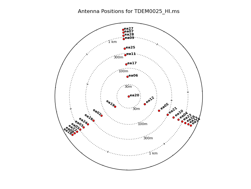
Using plotants, we'll look at the overall antenna layout and choose the best reference antenna based on certain criteria. We will want to choose a reference antenna that is closer to the center of the array, so any atmospheric changes are similar for all antennas. For D and C configuration, low declination sources are subject to antenna shadowing (which we will account for in the next section). Shadowed antennas will collect less radiation, causing lower sensitivity which may not be the best choice for the reference antenna. For this guide, we will use ea10 as the reference antenna.
# Interactive CASA
default plotants
inp
vis='TDEM0025.ms'
figfile='antlayout.png'
logpos=True
inp
go
# Psuedo-interactive CASA
plotants(vis='TDEM0025.ms',figfile='antlayout.png',logpos=True)
Step 4: Flag Antenna Shadowing and Zeros
Next we will use flagdata to flag any antennas that may have been shadowed during the observation. This is a necessary step when observing in D- or C-configuration. Once we set mode='shadow' more parameters become available to edit specific to antenna shadowing. We will leave those parameters as the default settings. Note, if an observation was taken in A- or B-configuration, this step is unnecessary.
# Interactive CASA
default flagdata
inp
vis='TDEM0025.ms'
mode='shadow'
inp
go
# Psuedo-interactive CASA
flagdata(vis='TDEM0025.ms', mode='shadow')
The correlator is known to generate a small number of zeros in the data. We will use flagdata to remove those zeros and to clip the very bright values. Setting mode='clip' in flagdata will reveal new parameters specific to this mode. We will leave most of the parameters as the default settings, however we will set two in particular: correlation='ABS_ALL' will take the absolute value of RR and LL and clip the very bright values and clipzeros=True will clip the zero-value data generated by the correlator.
# Interactive CASA
default flagdata
inp
vis='TDEM0025.ms'
mode='clip'
correlation='ABS_ALL'
clipzeros=True
inp
go
# Psuedo-interactive CASA
flagdata(vis='TDEM0025.ms', mode='clip', correlation='ABS_ALL', clipzeros=True)
More details regarding the use of flagdata can be found under the importasdm task.
Step 5: Split Out the HI Line
We only want to calibrate and image spw='0' since that is where we expect the line to be. So we will run split to create a new smaller MS containing only the HI line (spw 0).
# Interactive CASA
default split
inp
vis='TDEM0025.ms'
outputvis='TDEM0025_HI.ms'
spw=0
datacolumn='data'
inp
go
# Psuedo-interactive CASA
split(vis='TDEM0025.ms', outputvis='TDEM0025_HI.ms', spw=0, datacolumn='data')
If we run listobs on this new MS, we can see the output shows everything but the continuum spw's 1-8.
# Psuedo-interactive CASA
listobs(vis='TDEM0025_HI.ms', verbose=True, listfile='listobs_HI.txt')
Step 6: Inspecting and Flagging Bad Data
Before calibrating our dataset, it is important to inspect the initial data for any signs of faulty antennas or strong RFI. Prominent problems like these can easily be identified without calibrating the data, and flagging them now will prevent the need for re-calibration later on.
Antenna flagging
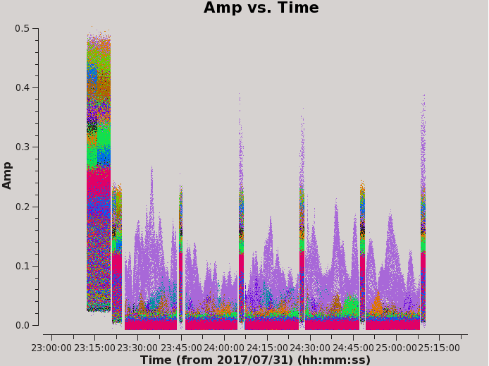
Let's look at amplitude variations with respect to time for each field. We will want to flag significant variations in amplitude and keep track of recurring antennas/timeframes/frequencies with abnormally high amplitude so these may be flagged as a collection of an issue.
By setting colors per baseline, we notice that one antenna is pretty noisy. Within the plotms GUI, click on the Mark Regions icon, select a few points of the widely varying amplitude, use the Locate icon (the magnifying glass) to output information on the data, and assess common details of the data. We notice that ea24 causes significant noise seen in Figure 3, where the purple data is ea24.
- Please keep in mind when using the flag icon in plotms, which is close to the locate icon, an automatic flagbackup is not set when interactively flagging.
# Interactive CASA
default plotms
inp
vis='TDEM0025_HI.ms'
xaxis='time'
yaxis='amp'
correlation='RR,LL'
selectdata=True
avgchannel='64'
coloraxis='baseline'
inp
go
# Psuedo-interactive CASA

plotms(vis='TDEM0025_HI.ms',xaxis='time',yaxis='amp',correlation='RR,LL',selectdata=True,avgchannel='64',coloraxis='baseline')
Where:
    vis='TDEM0025_HI.ms'          # the split HI ms
    xaxis='time'                  # plot time along the x axis
    yaxis='amp'                   # plot amplitude along the y axis
    correlation='RR,LL'           # plot the two parallel hand polarizations, Right and Left polarizations
    selectdata=True               # expand the parameters to choose from.
    avgchannel='64'               # average data every 64 channels
    coloraxis='baseline'          # colorize data points by baseline
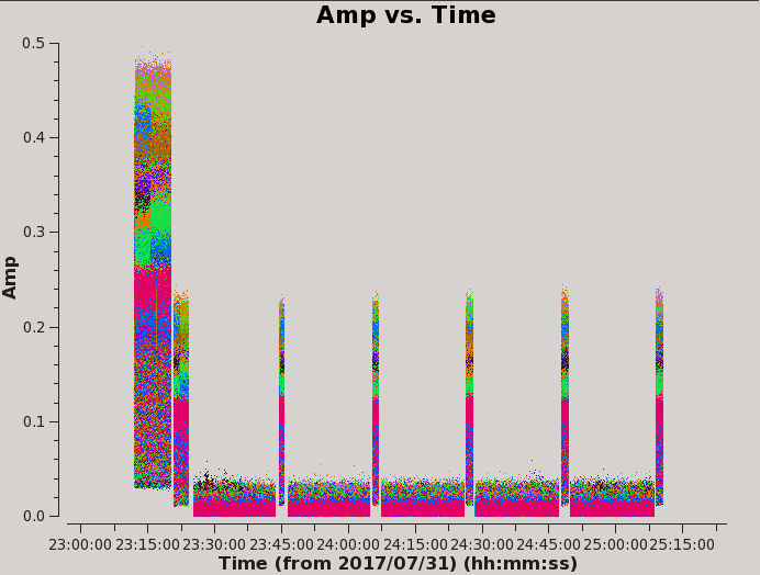
Within the Data tab exclude ea24 by typing !ea24 in the antenna selection. Re-plotting, we can see the overall amplitude is less variable as seen in Figure 4.
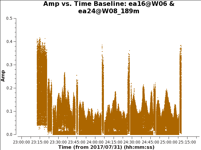
We can also iterate per baseline to the reference antenna ea10 and the suspected antenna ea24. by using the green arrow icon within plotms Here we notice that all baselines associated to ea24 vary in amplitude significantly. Figure 5 shows one baseline with ea16&ea24, and iterating through baselines with ea24 all show varying amplitudes.
# Interactive CASA
default plotms
inp
vis='TDEM0025_HI.ms'
xaxis='time'
yaxis='amp'
antenna='ea10,ea24'
correlation='RR,LL'
selectdata=True
avgchannel='64'
coloraxis='antenna1'
iteraxis='baseline'
inp
go
# Psuedo-interactive CASA

plotms(vis='TDEM0025_HI.ms',xaxis='time',yaxis='amp',antenna='ea10,ea24',correlation='RR,LL',selectdata=True,avgchannel='64',coloraxis='antenna1',iteraxis='baseline')
Where:
    vis='TDEM0025_HI.ms'          # the split HI ms.
    xaxis='time'                  # plot time along the x axis.
    yaxis='amp'                   # plot amplitude along the y axis.
    antenna='ea10,ea24'           # include antennas ea10 and ea24 only.
    correlation='RR,LL'           # plot the two parallel hand polarizations, Right and Left polarizations.
    selectdata=True               # expand the parameters to choose from.
    avgchannel='64'               # average data every 64 channels.
    coloraxis='antenna1'          # colorize by the first antenna.
    iteraxis='baseline'           # create a plot for each baseline to ea10 and ea24.
Now that we've narrowed down the noisy antenna, we will flag ea24 using flagdata which will also output to the casalogger the flagbackup version name.
# Interactive CASA
default flagdata
inp
vis='TDEM0025_HI.ms'
mode='manual'
antenna='ea24'
action='apply'
flagbackup=True
inp
go
# Psuedo-interactive CASA

flagdata(vis='TDEM0025_HI.ms',mode='manual',antenna='ea24',action='apply',flagbackup=True)
Where:
    vis='TDEM0025_HI.ms'      # the split HI ms
    mode='manual'             # flag data based on parameters specified.
    antenna='ea24'            # flag antennas and 24.
    action='apply'            # apply the flags to the ms.
    flagbackup=True           # automatically save flags into a predesignated flagversion name.
RFI flagging
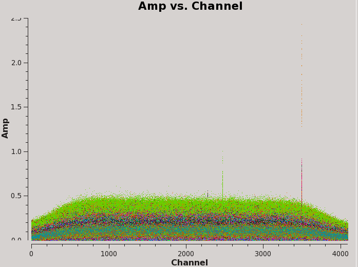
Now, let us have a look at amplitude vs. channel for the complex gain calibrator field.
# Interactive CASA
default plotms
inp
vis='TDEM0025_HI.ms'
field='1'
xaxis='channel'
yaxis='amp'
correlation='RR,LL'
coloraxis='antenna1'
inp
go
# Psuedo-interactive CASA
plotms(vis='TDEM0025_HI.ms', field='1', xaxis='channel', yaxis='amp', correlation='RR,LL', coloraxis='antenna1')
Figure 6 depicts that there is some strong RFI present in the data. If you use the interactive locate feature within plotms, you should discover that the largest RFI spike is localized to channel 3495 (spw='0:3495'). You can investigate further by interactively plotting a smaller region around this channel (i.e. spw='0:3200~3800') and setting iteraxis='antenna1'. By paging through the amplitude vs. channel plots of each antenna and using the locate feature on instances of RFI, you should discover that the RFI is only prevalent in baselines between antennas ea01, ea02, ea03, ea12, and ea16. We will flag this data.
Through the same methods, you should discover that the other two RFI spikes seen in Figure 6 belong to (almost all antennas in spw='0:2472~2473') and to (antennas ea01 and ea22 in spw='0:2281'). These should also be flagged.
# Interactive CASA

default flagdata
inp
vis='TDEM0025_HI.ms'
spw='0:3495'
antenna='ea01,ea02,ea03,ea12,ea16'
inp
go

#
spw='0:2472~2473'
antenna=''
inp
go


#
spw='0:2281'
antenna='ea01,ea22'
inp
go
# Psuedo-interactive CASA
flagdata(vis='TDEM0025_HI.ms', spw='0:3495', antenna='ea01,ea02,ea03,ea12,ea16')

flagdata(vis='TDEM0025_HI.ms', spw='0:2472~2473')

flagdata(vis='TDEM0025_HI.ms', spw='0:2281', antenna='ea01,ea22')
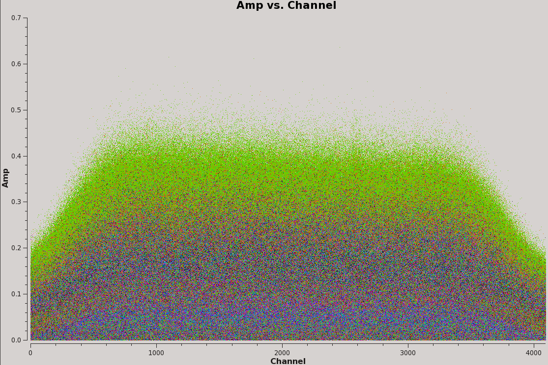
The RFI should now be completely flagged out (Figure 7).
Step 7: Initial Flux Density Scaling
Using setjy, we will list available models and set the model for the flux calibrator. By setting listmodels=True, setjy will show all available models for specific calibrators with specific bands in the Perley-Butler 2017 standard. setjy will look within the directory in which CASA was run for *.im *.mod files for user-defined models or images. If none are found, setjy will confirm this, for this particular dataset we will use a model in CalModels instead.
# Interactive CASA
default setjy
inp
vis='TDEM0025_HI.ms'
listmodels=True

inp
go
# Psuedo-interactive CASA
setjy(vis='TDEM0025_HI.ms',listmodels=True)
#terminal output
No candidate modimages matching '*.im* *.mod*' found in .  # The single period here refers to the current working directory.

Candidate modimages (*) in /home/casa/data/distro/nrao/VLA/CalModels:
3C138_A.im  3C138_L.im  3C138_U.im  3C147_C.im  3C147_Q.im  3C147_X.im  3C286_K.im  3C286_S.im  3C48_A.im  3C48_L.im  3C48_U.im
3C138_C.im  3C138_Q.im  3C138_X.im  3C147_K.im  3C147_S.im  3C286_A.im  3C286_L.im  3C286_U.im  3C48_C.im  3C48_Q.im  3C48_X.im
3C138_K.im  3C138_S.im  3C147_A.im  3C147_L.im  3C147_U.im  3C286_C.im  3C286_Q.im  3C286_X.im  3C48_K.im  3C48_S.im  README
Using setjy, we will set the model for the flux calibrator 3C286 (field='0') which was observed in L band.
# Interactive CASA
default setjy
inp
vis='TDEM0025_HI.ms'
listmodels=False
field='0'
spw='0'
scalebychan=True
fluxdensity=-1
standard='Perley-Butler 2017'
model='3C286_L.im'
usescratch=True
inp
go
# Psuedo-interactive CASA
setjy(vis='TDEM0025_HI.ms',listmodels=False,field='0',spw='0',scalebychan=True,fluxdensity=-1,standard='Perley-Butler 2017',model='3C286_L.im',usescratch=True)
Where:
    vis='TDEM0025_HI.ms'          # the split HI ms.
    listmodels='False'            # do not list the available models for VLA calibrators.
    field='0'                     # set the model for 3C286, the flux density calibrator for this observation.
    spw='0'                       # calculate the model for one spw.
    scalebychan=True              # set as default, the model is calculated per channel.
    fluxdensity=-1                # uses the flux density standard for recognized sources, and [1,0,0,0] for unrecognized.
    standard='Perley-Butler 2017' # Flux density standard used as the default.
    model='3C286_L.im'            # Use the L band model for 3C286.
    usescratch=True               # create a MODEL_DATA column containing model data
Within the casalogger, setjy outputs the flux in Janskys for Stokes I for a specific frequency.
2019-03-26 17:32:38 INFO imager	Using channel dependent flux densities
2019-03-26 17:32:38 INFO imager	Selected 68796 out of 831168 rows.
2019-03-26 17:32:38 INFO imager	1331+305=3C286 (fld ind 0) spw 0  [I=15.028, Q=0, U=0, V=0] Jy @ 1.4103e+09Hz, (Perley-Butler 2017)
2019-03-26 17:32:58 INFO imager	Using model image /home/casa/data/distro/nrao/VLA/CalModels/3C286_L.im
2019-03-26 17:32:58 INFO imager	Scaling spw(s) [0]'s model image by channel to  I = 15.0281, 14.9855, 14.9431 Jy @(1.41037e+09, 1.41838e+09, 1.42638e+09)Hz (LSRK) for visibility prediction (a few representative values are shown).
2019-03-26 17:32:58 INFO imager	The model image's reference pixel is 0.000254726 arcsec from 1331+305=3C286's phase center.
2019-03-26 17:32:58 INFO imager	Will clear any existing model with matching field=1331+305=3C286 and spw=*
2019-03-26 17:32:58 INFO  	Clearing model records in MS header for selected fields.
2019-03-26 17:32:58 INFO  	 1331+305=3C286 (id = 0) not found.
2019-03-26 17:32:58 INFO imager	Selected 68796 out of 831168 rows.
2019-03-26 17:32:58 INFO setjy	##### End Task: setjy                #####
2019-03-26 17:32:58 INFO setjy	##########################################
Step 8: Prior Calibration
In this step, we will solve for 'a priori' corrections. These include corrections for weather conditions during the observation, antenna positions, and antenna gain variability. We will summarize opacity corrections, ionospheric TEC corrections, and requantizer gain corrections and why they may not benefit this dataset.
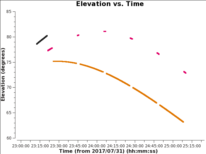
First, it is good to inspect the elevation of our sources since low elevation sources can be subject to antenna shadowing in C and D configurations. We have already flagged for shadowing in previous sections, but it helps to understand the location of our sources throughout the observation. Using plotms, we'll create an elevation versus time plot for all sources. The complex gain (amplitude and phase) calibrator should be closer to the target source to obtain a similar environment regarding changes in amplitude and phase which will be applied to the source.
# Interactive CASA
default plotms
inp
vis='TDEM0025_HI.ms'
xaxis='time'
yaxis='elevation'
correlation='RR,LL'
avgchannel='64'
coloraxis='field'
plotfile='elevstime.png'
inp
go
# Psuedo-interactive CASA
plotms(vis='TDEM0025_HI.ms',xaxis='time',yaxis='elevation',correlation='RR,LL',avgchannel='64',coloraxis='field',plotfile='elevstime.png')
Where:
    vis='TDEM0025_HI.ms'         # the split HI ms.
    xaxis='time'                 # plot time along the x axis.
    yaxis='elevation'            # plot elevation along the y axis.
    correlation='RR,LL'          # plot the two parallel hand polarizations, Right and Left polarizations.
    avgchannel='64'              # average data every 64 channels.
    coloraxis='field'            # colorize data points by field.
    plotfile='elevstime.png'     # automatically save this plot to a file titled elevstime.png.
Antenna gain-elevation curve calibration
With elevation, the effective collecting area and surface accuracy of antennas varies as gravity tugs at the surface of the non-rigid antenna. We know how to correct for this variation so by using gencal, we will write the gain curve solutions to a calibration table.
# Interactive CASA
default gencal
inp
vis='TDEM0025_HI.ms'
caltable='antgain.cal'
caltype='gc'
inp
go
# Psuedo-interactive CASA
gencal(vis='TDEM0025_HI.ms',caltable='antgain.cal',caltype='gc')
Where:
    vis='TDEM0025_HI.ms'   # the split HI ms.
    caltable='antgain.cal' # name of output calibration table where values are stored.
    caltype='gc'           # gain curve calculated per spw.
Opacities and weather conditions
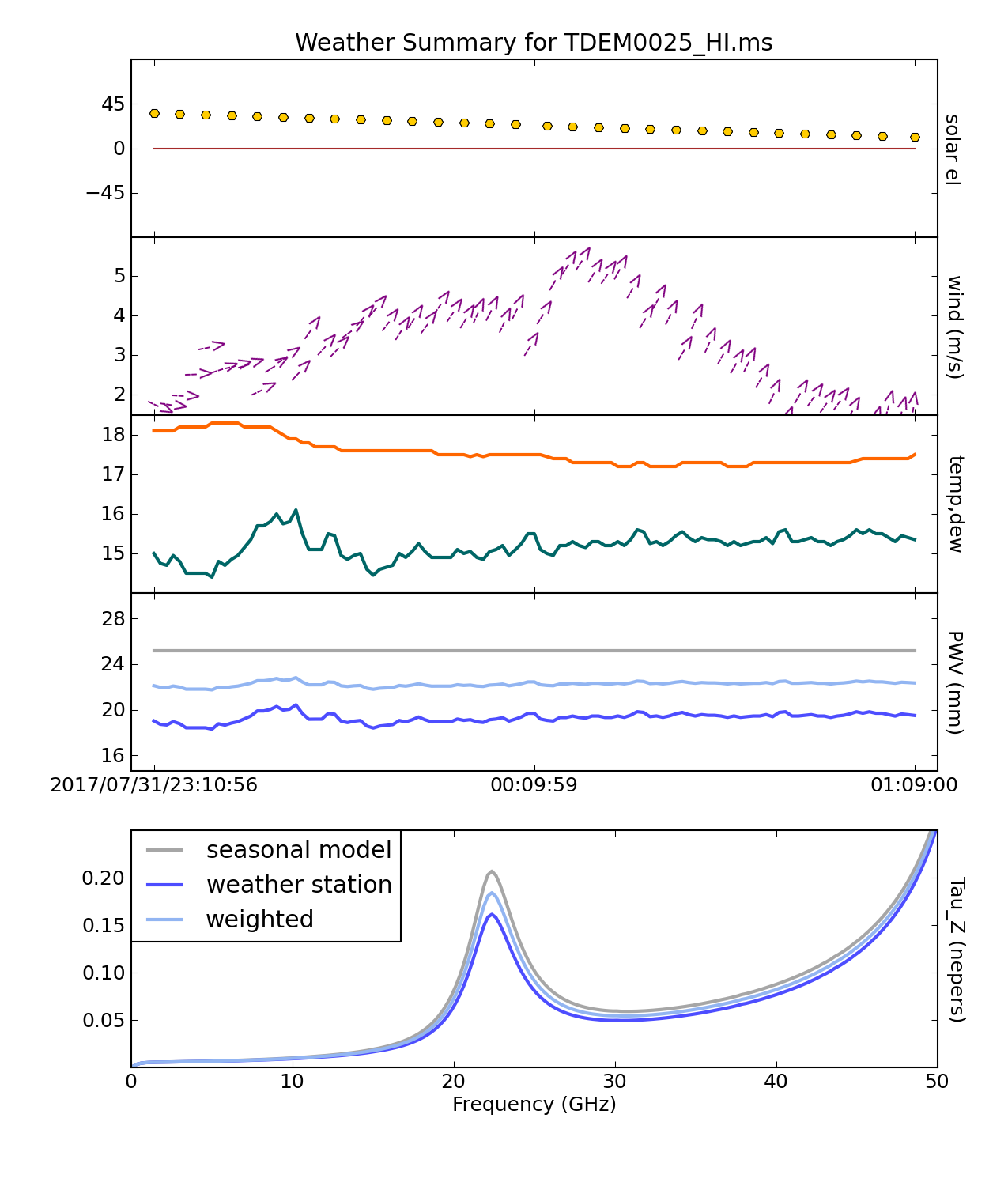
Using plotweather, we'll look at weather conditions throughout the observation that may affect the data. plotweather provides an estimate of the opacity on a per spw basis with units in nepers. The seasonal weight parameter calculates the opacities based on the weather data, seasonal model, or a combination of two. When the seasonal_weight is set to 1 the opacity corrections are derived using only the seasonal data and when set to 0 the opacity corrections are derived from only the weather data.
Atmospheric opacity attenuates incoming radiation and observations at different elevations affect the flux density scale of sources. For lower frequency observation (Ku and lower), this attenuation is small and opacity corrections are usually skipped. Luckily for L band, weather conditions do not significantly affect (unless it’s snow, rain, or strong winds) the data, therefore we can save the weather plots for reference and skip opacity corrections.
# Interactive CASA
default plotweather
inp
vis='TDEM0025_HI.ms'
seasonal_weight=0.5
plotName='TDEM0025weathercond.png'
doPlot=True
inp
go
# Psuedo-interactive CASA
plotweather(vis='TDEM0025_HI.ms',seasonal_weight=0.5,plotName='TDEM0025weathercond.png',doPlot=True)
Where:
    vis='TDEM0025_HI.ms'                         # the split HI ms.
    seasonal_weight=0.5                          # calculate opacities using both the seasonal model and weather data.
    plotName='TDEM0025weathercond.png'           # name of the generated plot
    doPlot=True                                  # create plot. If set to false, do not create plot and output only the calculated opacities.
Requantizer gains calibration
Requantizer gain corrections account for gain changes that occur when resetting the quantizer gains as the correlator changes to a new 3-bit configuration. Requantizer gains need to be redetermined after a change of tuning. To create a calibration table containing corrections for the requantizer gains one would use gencal with caltype=’rq’. However, since this observation uses 8-bit setup this step can be skipped. For information on 8 bit, 3 bit setup observations, and requantizer setup scans here is a link to 8/3-Bit Attenuator and Requantizer Gain Setup Scans
Ionopsheric TEC calibration
The Total Electron Content (TEC) is the total number of electrons present along a path between a radio source and receiver. Ionospheric corrections are important for frequencies below 1GHz or for polarimetry. For this guide, we will not derive or apply TEC corrections.
Antenna position corrections
We will calculate antenna position corrections using gencal which queries the VLA Archive: Baseline Corrections.
# Interactive CASA
default gencal
inp
vis='TDEM0025_HI.ms'
caltype='antpos'
caltable='antpos.cal'
antenna=''
inp
go
# Psuedo-interactive CASA
gencal(vis='TDEM0025_HI.ms',caltype='antpos',caltable='antpos.cal',antenna='')
Where:
    vis='TDEM0025_HI.ms'   # the split HI ms
    caltype='antpos'       # the type of calibration to solve for, where antpos gathers the ITRF antenna position offsets
    caltable='antpos.cal'  # create a calibration table titled antpos.cal where the antenna position offsets can be stored
    antenna=''             # search for all antennas
gencal will report into the casalogger, if there are any antenna position corrections found. In this case, there are position corrections for antenna ea25 that are saved into the calibration table antpos.cal and will be applied in later stages using applycal and gaincal.
- Please note gencal will also report to the logger if there are no antenna position corrections for the observation. This simply means all antenna position corrections were applied by the VLA Operator before the science observation was made.
2019-03-25 21:52:22	INFO	gencal::::+	##########################################
2019-03-25 21:52:22	INFO	gencal::::+	##### Begin Task: gencal             #####
2019-03-25 21:52:22	INFO	gencal::::	gencal(vis="TDEM0025_HI.ms",caltable="antpos.cal",caltype="antpos",infile="",spw="",
2019-03-25 21:52:22	INFO	gencal::::+	        antenna="",pol="",parameter=[],uniform=True)
2019-03-25 21:52:22	INFO	calibrater::open	****Using NEW VI2-driven calibrater tool****
2019-03-25 21:52:22	INFO	calibrater::open	Opening MS: TDEM0025_HI.ms for calibration.
2019-03-25 21:52:22	INFO	Calibrater::	Initializing nominal selection to the whole MS.
2019-03-25 21:52:22	INFO	gencal::::	 Determine antenna position offsets from the baseline correction database
2019-03-25 21:52:22	INFO	gencal::::	offsets for antenna ea25 : -0.00200   0.00000  -0.00120
2019-03-25 21:52:22	INFO	calibrater::specifycal	Beginning specifycal-----------------------
2019-03-25 21:52:22	INFO		Creating KAntPos Jones table from specified parameters.
2019-03-25 21:52:22	INFO		Writing solutions to table: antpos.cal
2019-03-25 21:52:22	INFO	gencal::::	##### End Task: gencal               #####
Step 9: Bandpass Calibration, Complex Gain Calibration, and Fluxscale
Bandpass Calibration
Now, we can run our bandpass calibration. This calibration gives antenna-based solutions against a reference antenna. This will determine the variations of phase and amplitude across frequency for this calibrator. Once we have solutions, we can then correct for these variations on the complex gain calibrator and the target.
# Interactive CASA
default bandpass
inp
vis='TDEM0025_HI.ms'
caltable='bandpass.cal'
field='0'
refant='ea10'
solint='inf'
gaintable=['antgain.cal','antpos.cal']
inp
go
# Psuedo-interactive CASA

bandpass(vis='TDEM0025_HI.ms',caltable='bandpass.cal',field='0',refant='ea10',solint='inf',gaintable=['antgain.cal','antpos.cal'])
Where:
    vis='TDEM0025_HI.ms'                     # the split HI ms
    caltable='bandpass.cal'                  # the name you wish to give the calibration table
    field='0'                                # the field id of the bandpass calibrator (or you could give it the field name)
    refant='ea10'                            # the reference antenna you have chosen
    solint='inf'                             # the solution interval time
    gaintable=['antgain.cal','antpos.cal']   # gain calibration table(s) to apply on the fly
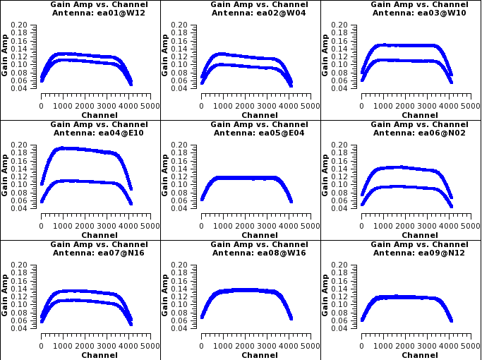
Now we will plot the bandpass solutions as phase vs channel and amplitude vs channel per antenna. Start with looking at the amplitudes. These should be smooth across the channels. You will see the edge channels have lower amplitudes due to the edges, of the spw, being less sensitive. This sensitivity loss is a property of the hardware and is dependent on frequency.
# Interactive CASA
default plotms
inp
vis='bandpass.cal'
xaxis='chan'
yaxis='amp'
iteraxis='antenna'
gridrows=3
gridcols=3
xselfscale=True
yselfscale=True
inp
go
# Psuedo-interactive CASA

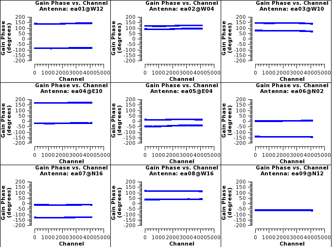
plotms(vis='bandpass.cal',xaxis='chan',yaxis='amp',iteraxis='antenna',gridrows=3,gridcols=3,xselfscale=True,yselfscale=True)
Where:
    vis='bandpass.cal'    # the bandpass calibration table
    xaxis='chan'          # plot channels across the x axis
    yaxis='amp'           # plot amplitudes across the y axis
    iteraxis='antenna'    # pages the plots by antenna
    gridrows=3            # places 3 antennas per row
    gridcols=3            # places 3 antennas per column
    xselfscale=True       # create a global xaxis scale for all antennas
    yselfscale=True       # create a global yaxis scale for all antennas
You may see the phases vs channel by changing the yaxis to phase interactively. The phases should be relatively flat and continuous.
Complex Gain Calibration
Next we will calibrate the amplitude and phases of the data using the bandpass and complex gain calibrators. To do this we will use gaincal and the previously made calibration tables. This will give us antenna based solutions that will show variations across time.
# Interactive CASA
default gaincal
inp
vis='TDEM0025_HI.ms'
caltable='apcal.gcal'
field='0,1'
refant='ea10'
calmode='ap'
solint='inf'
minsnr=3.0
gaintable=['antgain.cal','antpos.cal','bandpass.cal']
inp
go
# Psuedo-interactive CASA

gaincal(vis='TDEM0025_HI.ms',caltable='apcal.gcal',field='0,1',refant='ea10',calmode='ap',solint='inf',minsnr=3.0,gaintable=['antgain.cal','antpos.cal','bandpass.cal'])
Where:
    vis='TDEM0025_HI.ms'                                    # the split HI ms
    caltable='apcal.gcal'                                   # the name you wish to give the calibration table
    field='0,1'                                             # the field id of the bandpass calibrator (or you could give it the field name)
    refant='ea10'                                           # the reference antenna you have chosen
    calmode='ap'                                            # the calibration mode that finds both amplitude and phase solutions
    solint='inf'                                            # the solution interval time
    minsnr=3.0                                              # the minimum signal to noise ratio to reject solutions
    gaintable=['antgain.cal','antpos.cal','bandpass.cal']   # gain calibration table(s) to apply on the fly
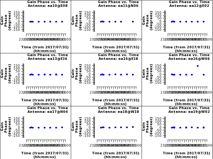
Now look at solutions. First we will look at the phase solutions. These should be at zero with no phase jumps; phase jumps are when the phases change drastically with time. When this happens we are not able to interpolate the phases surrounding that scan that has the phase jump.
# Interactive CASA
default plotms
inp
vis='apcal.gcal'
xaxis='time'
yaxis='phase'
iteraxis='antenna'
gridrows=3
gridcols=3
plotrange=[0,0,-180,180]
inp
go
# Psuedo-interactive CASA

plotms(vis='apcal.gcal',xaxis='time',yaxis='phase',iteraxis='antenna',gridrows=3,gridcols=3,plotrange=[0,0,-180,180])
Where:
    vis='apcal.gcal'              # the complex gain calibration table
    xaxis='time'                  # plot channels across the x axis
    yaxis='phase'                 # plot amplitudes across the y axis
    iteraxis='antenna'            # pages the plots by antenna
    gridrows=3                    # places 3 antennas per row
    gridcols=3                    # places 3 antennas per column
    plotrange=[0,0,-180,180]      # sets the plot range
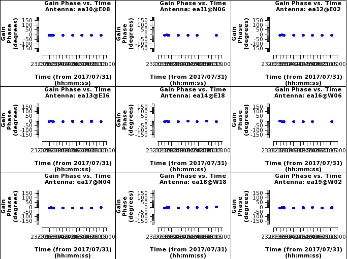
Pressing next through these phase vs time plot we can see that antenna ea16 and ea20 have a scan that shows a phase jump relative to the rest of the scans. If we locate this point we see that it is scan 21 for both antennas. This scan we should flag so that the target scans surrounding that calibrator scan will have correct phase solutions applied to them.
Now look at the amplitudes to see if there are any other irregularities.
# Interactive CASA
default plotms
inp
vis='apcal.gcal'
xaxis='time'
yaxis='amp'
iteraxis='antenna'
gridrows=3
gridcols=3
xselfscale=True
yselfscale=True
inp
go
# Psuedo-interactive CASA

plotms(vis='apcal.gcal',xaxis='time',yaxis='amp',iteraxis='antenna',gridrows=3,gridcols=3,xselfscale=True,yselfscale=True)
Where:
    vis='apcal.gcal'         # the complex gain calibration table
    xaxis='time'             # plot channels across the x axis
    yaxis='amp'              # plot amplitudes across the y axis
    iteraxis='antenna'       # pages the plots by antenna
    gridrows=3               # places 3 antennas per row
    gridcols=3               # places 3 antennas per column
    xselfscale=True          # create a global xaxis scale for all antennas
    yselfscale=True          # create a global yaxis scale for all antennas
Seeing no other things to be concerned about, we will flag the antennas affected by the phase jump and then rederive the amplitude and phase gaincal solutions.
# Interactive CASA
default flagdata
inp
vis='TDEM0025_HI.ms'
mode='manual'
antenna='ea16,ea20'
scan='21'
action='apply'
flagbackup=True
inp
go
# Psuedo-interactive CASA

flagdata(vis='TDEM0025_HI.ms',mode='manual',antenna='ea16,ea20',scan='21',action='apply',flagbackup=True)
Where:
    vis='TDEM0025_HI.ms'   # the split HI ms
    mode='manual'          # flag data based on parameters specified.
    antenna='ea16,ea20'    # flag only antennas ea16 and ea20
    scan='21'              # flag only scan 21 for both antennas
    action='apply'         # apply the flags to the split HI ms.
    flagbackup=True        # automatically save flags into a predesignated flagversion name.
Now you should rerun the gaincal step that created the apcal.gcal table and the phase plotms runs from above. This will rederive the solutions and then you can see that scan 21 for both ea16 and ea20 have been flagged.
Note: we are able to flag this calibration scan and not have to flag any of the surrounding target scans because of the cycle time recommended for L band in the C configuration. Where the cycle time is ~40 minutes. The time between the 2 complex gain calibrator scans surrounding scan 21 is ~43 minutes. It is lucky that the observation was set up to have a shorter cycle time than recommended or else we would have to flag all of the scans between calibrator scans 17 and 25 which would have gotten rid of 2/5 of our data set.
Fluxscale
Now that calibration of the observation seems to be done we will use fluxscale to calculate the amplitude of the complex gain calibrator. We can do this because we know the amplitude of the flux density scale/bandpass calibrator. We do this by referencing the flux density scale/bandpass calibrator and applying the calibration table solutions we just derived.
# Interactive CASA
default fluxscale
inp
vis='TDEM0025_HI.ms'
caltable='apcal.gcal'
reference='0'
fluxtable='flux_scale.cal'
incremental=True
inp
go
# Psuedo-interactive CASA

fluxscale(vis='TDEM0025_HI.ms',caltable='apcal.gcal',reference='0',fluxtable='flux_scale.cal',incremental=True)
Where:
    vis='TDEM0025_HI.ms'           # the split HI ms
    caltable='apcal.gcal'          # the calibration table used to find amplitude and phase corrections
    reference='0'                  # the field ID of the reference field (where you transfer  your flux from)
    fluxtable='flux_scale.cal'     # the name of the output, flux-scaled calibration table
    incremental=True               # creates a separate fluxscale table rather than edit the apcal.gcal table
This is the output to the terminal you will see when you run fluxscale. We will applies this to both the complex gain calibrator and the target in the next steps.
{'1': {'0': {'fluxd': array([ 6.91913842,  0.        ,  0.        ,  0.        ]),
   'fluxdErr': array([ 0.00403804,  0.        ,  0.        ,  0.        ]),
   'numSol': array([ 52.,   0.,   0.,   0.])},
  'fieldName': 'J1330+2509',
  'fitFluxd': 0.0,
  'fitFluxdErr': 0.0,
  'fitRefFreq': 0.0,
  'spidx': array([ 0.,  0.,  0.]),
  'spidxerr': array([ 0.,  0.,  0.])},
 'freq': array([  1.41832755e+09]),
 'spwID': array([0], dtype=int32),
 'spwName': array(['EVLA_L#A0C0#0'],
       dtype='|S14')}
Reading through this output you can see that for spw 0 the flux of the complex gain calibrator is ~6.919Jy. This is very close to the expected value of 6.80Jy in L-band. This expected value can be found by looking in the VLA Calibrator Manual, which you can google, and searching for the source.
Step 10: Applying the Calibration and Inspecting the Data
Applycal
Now that we have derived the appropriate calibration tables, we can apply these corrections to both our calibrator sources and target sources using the CASA task applycal, which creates a corrected data column where the calibrated data are stored. We apply the antenna position, antenna gaincurve, bandpass, complex gain, and fluxscale corrections to each field while specifying which source was used to derive each correction. For our flux/bandpass calibrator 3C286 (field='0') the applycal task looks like this:
# Interactive CASA
default applycal
inp
vis='TDEM0025_HI.ms'
field='0'
gaintable=['antgain.cal', 'antpos.cal', 'bandpass.cal', 'apcal.gcal', 'flux_scale.cal']
gainfield=['','','0','0','0']
calwt=False
flagbackup=True
inp
go
# Psuedo-interactive CASA

# for the flux/bandpass calibrator (field '0')
applycal(vis='TDEM0025_HI.ms', field='0',
         gaintable=['antgain.cal', 'antpos.cal', 'bandpass.cal', 'apcal.gcal', 'flux_scale.cal'],
         gainfield=['','','0','0','0'],
         calwt=False, flagbackup=True)
Where:
    vis='TDEM0025_HI.ms'                                                                         # the split HI ms
    field='0'                                                                                    # field id(s) or field name(s) for corrections to be applied to
    gaintable=['antgain.cal','antpos.cal','bandpass.cal','apcal.gcal','flux_scale.cal']           # gain calibration table(s) to apply on the fly
    gainfield=['','','0','0','0']                                                                # field id(s) from which each respective gaintable was derived
    calwt=False                                                                                  # determines if the weights are calibrated along with the data
    flagbackup=True                                                                              # automatically back up the state of flags before the run
Within the gainfield parameter, we did not specify a field for the first two tables ('antgain.cal', 'antpos.cal') since these were derived independently from our calibrator fields. For the calibrators, all bandpass solutions are the same as for the bandpass calibrator (id=0), and the phase and amplitude calibration as derived from their own visibility data. So when applying corrections to any of our sources, the respective field for 'bandpass.cal' will be our bandpass calibrator (field='0').
# Interactive CASA

# for the phase calibrator (field '1')
default applycal
inp
vis='TDEM0025_HI.ms'
field='1'
gaintable=['antgain.cal', 'antpos.cal', 'bandpass.cal', 'apcal.gcal', 'flux_scale.cal']
gainfield=['','','0','1','1']
calwt=False
flagbackup=True
inp
go

# for the target (field '2')
default applycal
inp
vis='TDEM0025_HI.ms'
field='1'
gaintable=['antgain.cal', 'antpos.cal', 'bandpass.cal', 'apcal.gcal', 'flux_scale.cal']
gainfield=['','','0','1','1']
calwt=False
flagbackup=True
inp
go
# Psuedo-interactive CASA

# for the phase calibrator (field '1')
applycal(vis='TDEM0025_HI.ms', field='1',
         gaintable=['antgain.cal', 'antpos.cal', 'bandpass.cal', 'apcal.gcal', 'flux_scale.cal'],
         gainfield=['','','0','1','1'],
         calwt=False, flagbackup=True)

# for the target (field '2')
applycal(vis='TDEM0025_HI.ms', field='2',
         gaintable=['antgain.cal', 'antpos.cal', 'bandpass.cal', 'apcal.gcal', 'flux_scale.cal'],
         gainfield=['','','0','1','1'],
         calwt=False, flagbackup=True)
As you can see we specify the bandpass calibrator (field '0') respectively with the 'bandpass.cal' table, regardless of which source we are correcting. The 'apcal.gcal' table is linked to the complex gain calibrator (field '1'), and the 'flux_scale' correction, which was derived from 'apcal.gcal', is also linked to the complex gain calibrator.
Inspect the Data
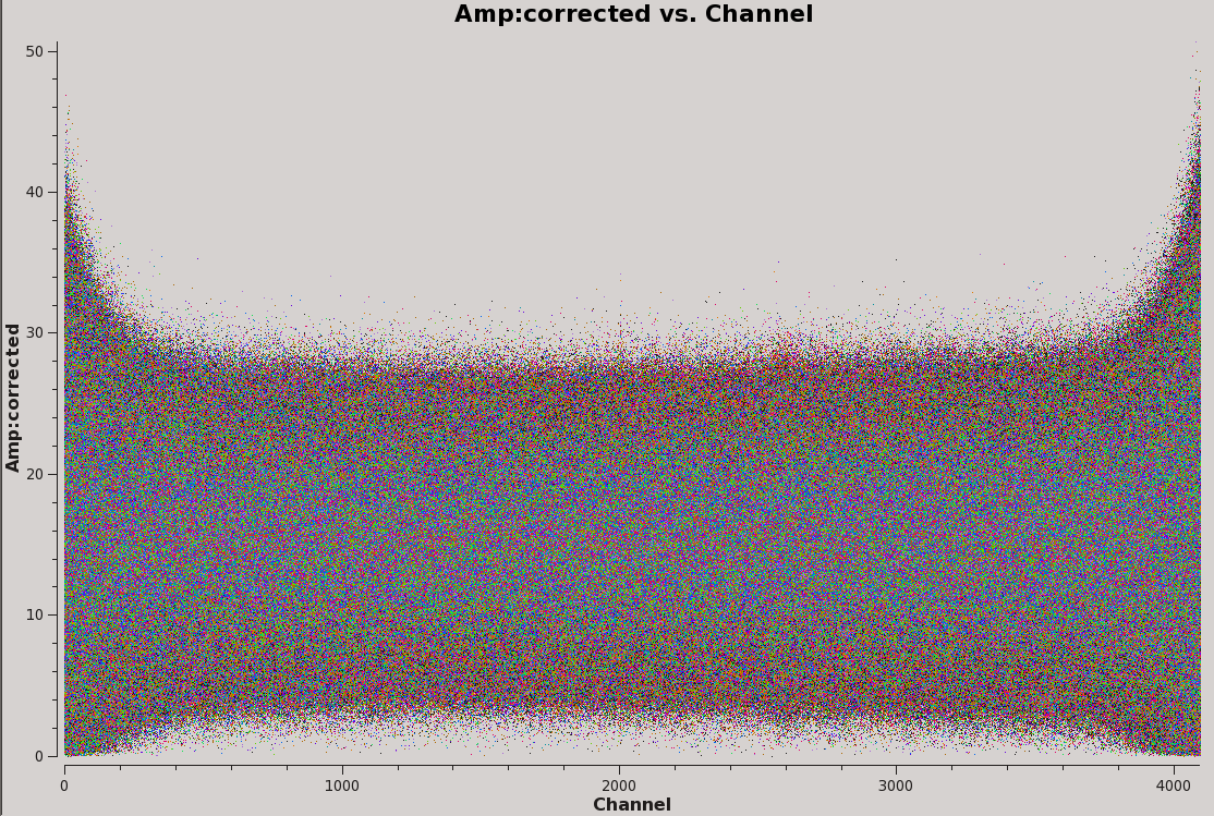
We have now applied our corrections, and can inspect the resulting data. The applycal task stores the calibrated data in a corrected data column within the MS and we can view this by specifying 'ydatacolumn' in plotms. First, let us have a look at amplitude vs. channel for the bandpass calibrator.
# Interactive CASA
default plotms
inp
vis='TDEM0025_HI.ms'
field='0'
xaxis='channel'
yaxis='amp'
ydatacolumn='corrected'
correlation='RR,LL'
coloraxis='antenna1'
inp
go
# Psuedo-interactive CASA
plotms(vis='TDEM0025_HI.ms', field='0', xaxis='channel', yaxis='amp', ydatacolumn='corrected', correlation='RR,LL', coloraxis='antenna1')
In addition to this, you can inspect other plots such as amplitude vs. time, phase vs. channel/time, amplitude vs. UVwave, etc.. If you find any residual RFI or outlying points that need flagging, flag the data and then go back and re-calibrate starting from the bandpass calibration step. Then, re-apply the calibrations as we have done above. It may be helpful to append your redone calibration tables with something like '_redo' in order to keep track of versions. In our case however, the data looks good and there is no need for further flagging or re-calibration.
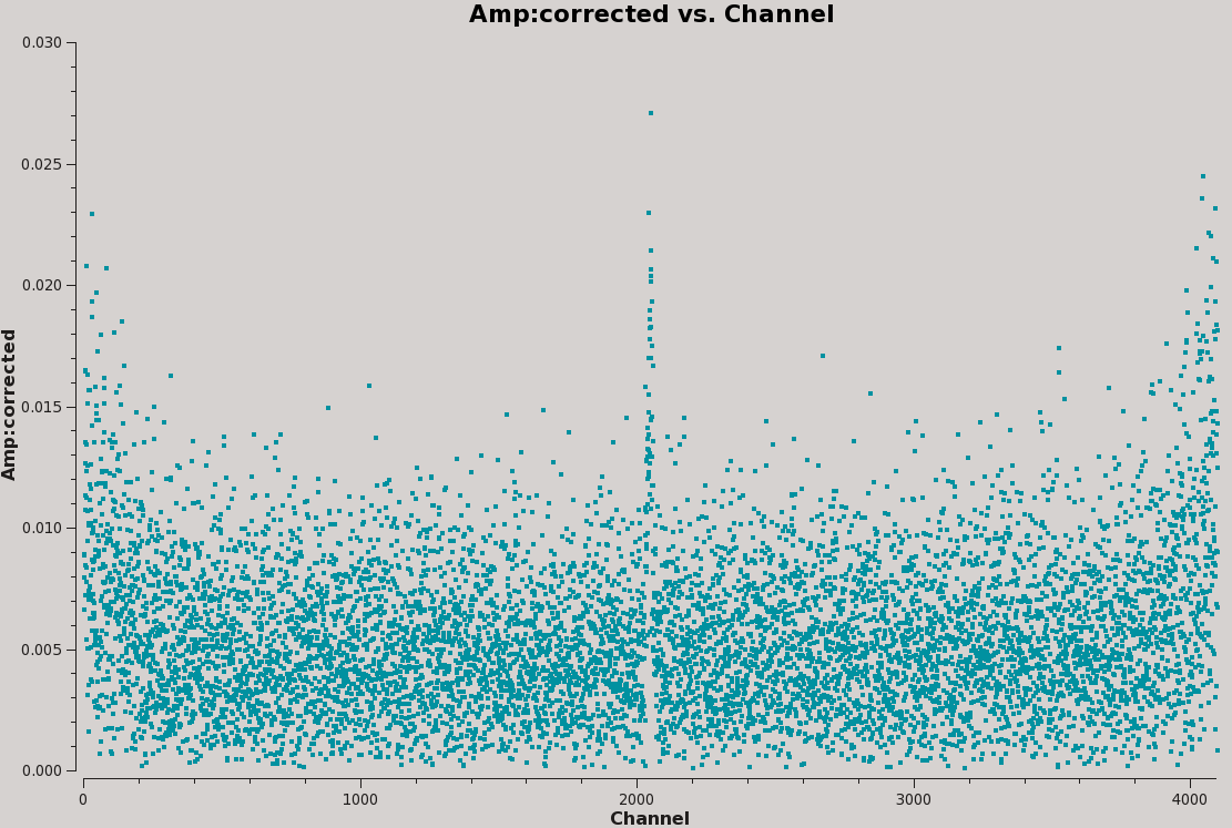
Now that our data set is calibrated, we can take a first glance at where the HI spectral line might be. Although we will obtain a highly resolved spectra later during the imaging section, it is useful to plot the our MS while averaging over all baselines and scans. This will make the spectral line easier to see and allow us to get a good idea of what channels it occupies, as well as serve as a sanity check that our calibration went well (Figure 15).
# Interactive CASA
default plotms
inp
vis='TDEM0025_HI.ms'
field='2'
xaxis='channel'
yaxis='amp'
ydatacolumn='corrected'
correlation='RR,LL'
coloraxis='antenna1'
avgtime='1e6'
avgscan=True
avgbaseline=True
inp
go
# Psuedo-interactive CASA
plotms(vis='TDEM0025_HI.ms', field='2', xaxis='channel', yaxis='amp', ydatacolumn='corrected', correlation='RR,LL', coloraxis='antenna1', avgtime='1e6', avgscan=True, avgbaseline=True)
Split
This procedure, although not necessary, is useful because it allows us to return to this point if we make a mistake or get confused in later processing. It also makes smaller individual files in case you want to copy to another machine or want to share the data with a colleague. Here we will split off the corrected data for the target field (field '2'), which will be placed in the data column of the new MS.
# Interactive CASA
default split
inp
vis='TDEM0025_HI.ms'
outputvis='TDEM0025_target_corrected.ms'
field='2'
datacolumn='corrected'
inp
go
# Psuedo-interactive CASA
split(vis='TDEM0025_HI.ms', outputvis='TDEM0025_target_corrected.ms', field='2', datacolumn='corrected')
Step 11: Imaging with tclean
Now we are ready to create the first image of our target. This is done with the CASA task tclean. Before creating an image cube of all 4096 channels, we will start by cleaning a single line-free channel so that we can determine which parameters to use. Specifically, we would like to determine a cleaning threshold to use when creating our full image cube.
The HPBW for C - Configuration, L -Band Observation is expected to be about 20 arcsec when assuming natural weighting. For the most effective cleaning we recommend using a pixel size such that there are 3 - 5 pixels across the synthesized beam. Thus, based on the assumed synthesized beam size of 20 arcsec, we will use a cell (pixel) size of 4.0 arcsec.
Additionally, as a general guideline we recommend image sizes [math]\displaystyle{ 2^n*10 }[/math] pixels, e.g. 160, 1280 pixels, etc. for improved processing speeds. Here we will use n=5 or imsize=[320,320]. With this, we can begin interactively cleaning a single channel.
Note: Since we are creating an image cube with only one channel, you should set nchan=1.
Interactive cleaning
# Interactive CASA
default tclean
inp
vis='TDEM0025_target_corrected.ms'
imagename='TDEM0025_target_initial_clean'
datacolumn='data'
specmode='cube'
spw='0:3000'
niter=1
cell=['4.0arcsec','4.0arcsec']
imsize=[320,320]
nchan=1
interactive=True
inp
go
# Psuedo-interactive CASA
tclean(vis='TDEM0025_target_corrected.ms', imagename='TDEM0025_target_initial_clean',
datacolumn='data', specmode='cube', spw='0:3000', niter=1, cell=['4.0arcsec','4.0arcsec'], imsize=[320,320], nchan=1, interactive=True)
Where:

    vis='TDEM0025_target_corrected.ms'                    # the split target ms
    imagename='TDEM0025_target_initial_clean'             # the name of ouput images
    datacolumn='data'                                     # using the data column of the split ms
    specmode='cube'                                       # creating an image cube
    spw='0:3000'                                          # we are cleaning a single line-free channel
    niter=1                                               # niter cannot be 0 to run interactive clean
    cell=['4.0arcsec','4.0arcsec']                        # cell/pixel size
    imsize=[320,320]                                      # image size in arcsec
    nchan=1                                               # number of channels we are making the cube with
    interactive=True                                      # interactive cleaning
Here we specified niter=1 because we would like to begin cleaning from the dirty image (niter=0), however tclean will not open the interactive clean GUI if the number of iterations is zero. It will take a little while to grid the data, but the viewer will open when it's ready to start an interactive clean.
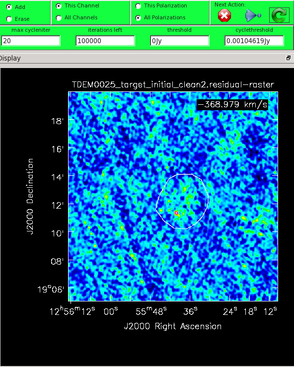
In the green menu on top, select 'this channel' (this is a bit redundant since we are only cleaning one channel) and all polarizations for the clean mask. Select the polygon tool ![]() and draw a border around the area in which you wish to mask. The lines drawn by the polygon tool will be green, making it difficult to see on a green image. You can change the color map under the Data Display Options (click on the wrench icon or in the top menu, select Data, then select Adjust Data Display). In the image, make a single mask by clicking on the image to drop anchor points and drawing lines between the points; double click for the last point after which the anchor points can be adjusted (be careful not to click outside as that removes the polygon). Once the polygon region is satisfactory, double click inside it to save the mask region. The polygon will then turn white (see Figure 16). Note, that if we had the time and patience, we could make a clean mask for each channel, and this would create a slightly better result.
and draw a border around the area in which you wish to mask. The lines drawn by the polygon tool will be green, making it difficult to see on a green image. You can change the color map under the Data Display Options (click on the wrench icon or in the top menu, select Data, then select Adjust Data Display). In the image, make a single mask by clicking on the image to drop anchor points and drawing lines between the points; double click for the last point after which the anchor points can be adjusted (be careful not to click outside as that removes the polygon). Once the polygon region is satisfactory, double click inside it to save the mask region. The polygon will then turn white (see Figure 16). Note, that if we had the time and patience, we could make a clean mask for each channel, and this would create a slightly better result.
If you need to include more area in the mask, you can choose the erase toggle at the top, and then encircle your existing mask with a polygon and double click inside. Then switch back to the add toggle at top and make a new mask. Alternatively, you can erase a part of the mask, or you can add to the existing mask by drawing new polygons. Feel free to experiment with these tools.
The mask you see in Figure 16 was drawn with some foresight in that the HI emission resides above the bright point source. To continue with tclean, we will set the 'iterations left' parameter to some arbitrarily large number. This limits the total number of minor cycles run within the CLEAN algorithm. The 'max cycleniter' parameter specifies the number of minor cycles per major cycle. To start, let us pick a modest number of 20. Use one of the Next action buttons in the green area on the Viewer Display GUI: The red X ![]() will stop tclean where it is; the blue arrow
will stop tclean where it is; the blue arrow ![]() will stop the interactive part of tclean, but continue to clean non-interactively until reaching the stopping niter (iterations left) or threshold, whichever comes first. The green arrow
will stop the interactive part of tclean, but continue to clean non-interactively until reaching the stopping niter (iterations left) or threshold, whichever comes first. The green arrow ![]() will clean until it reaches the max cycleniter parameter on the left side of the green area (1 major cycle).
will clean until it reaches the max cycleniter parameter on the left side of the green area (1 major cycle).
With our selected parameters, press the green arrow ![]() to begin cleaning. The buttons within the interactive GUI will grey out until the 20 minor cycles have completed. When the interactive viewer comes back, inspect the resulting residual image by adjusting the color scale (if your mouse has a middle button, then by default it controls the image stretch). Your goal should be to clean until the entire image, including the area within the mask, looks like uniform noise.
to begin cleaning. The buttons within the interactive GUI will grey out until the 20 minor cycles have completed. When the interactive viewer comes back, inspect the resulting residual image by adjusting the color scale (if your mouse has a middle button, then by default it controls the image stretch). Your goal should be to clean until the entire image, including the area within the mask, looks like uniform noise.
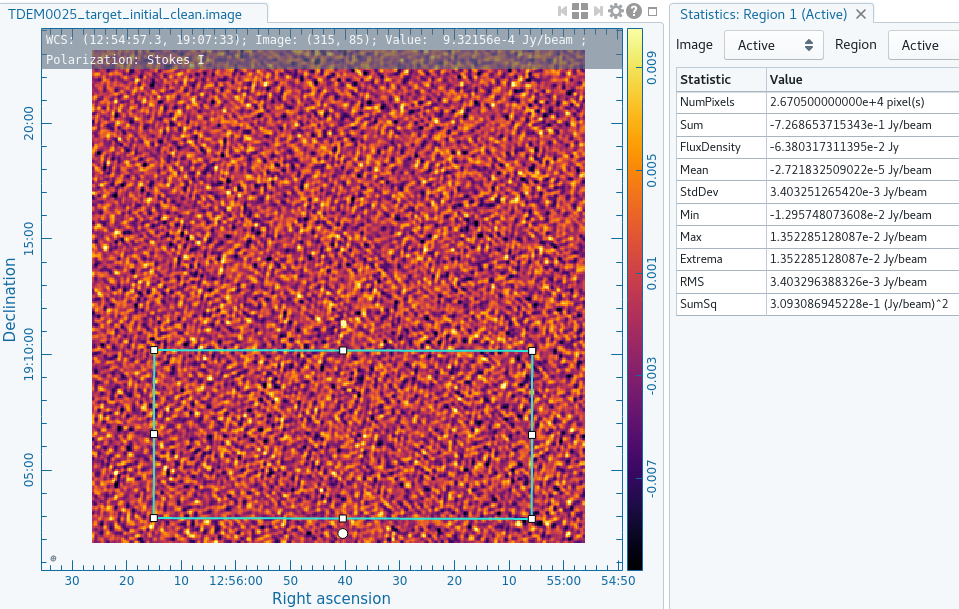
Once you are satisfied that the image has been cleaned sufficiently, exit tclean with the red X ![]() . You should view your cleaned image using the viewer task by simply typing viewer() in terminal and selecting the raster image of your cleaned image. For our purposes, this is named TDEM0025_target_initial_clean.image. In the viewer GUI, use the rectangular region tool
. You should view your cleaned image using the viewer task by simply typing viewer() in terminal and selecting the raster image of your cleaned image. For our purposes, this is named TDEM0025_target_initial_clean.image. In the viewer GUI, use the rectangular region tool ![]() to select an area that covers a large amount of the surrounding noise but does not include the source (Figure 17). Then, go to the Statistics tab under the Region properties and record what the RMS is. Here, our image shows an RMS of about 0.0029Jy. We will use this value in the next step to create our full, 4096 channel image cube.
to select an area that covers a large amount of the surrounding noise but does not include the source (Figure 17). Then, go to the Statistics tab under the Region properties and record what the RMS is. Here, our image shows an RMS of about 0.0029Jy. We will use this value in the next step to create our full, 4096 channel image cube.
Full image cube
Interactively cleaning all 4096 channels would obviously be intensive. So, we will want to do this automatically by specifying a threshold stopping criterion. In the previous step, we found that the average RMS of our image was about 0.0029Jy. Taking the 4σ of these noise levels (about 0.0116Jy) gives us a good threshold to work with. We now run tclean automatically on all of our channels, letting it clean until it reaches the threshold. Again, let the 'niter' parameter be some arbitrarily large number to ensure the threshold is reached.
# Interactive CASA
default tclean
inp
vis='TDEM0025_target_corrected.ms'
imagename='TDEM0025_target_full_clean'
datacolumn='data'
specmode='cube'
niter=1000000
threshold='0.0116Jy'
cell=['3.0arcsec','3.0arcsec']
imsize=[320,320]
outframe='bary'
veltype='optical'
restfreq='1420.405752MHz'
robust=0.3
inp
go
# Psuedo-interactive CASA
tclean(vis='TDEM0025_target_corrected.ms', imagename='TDEM0025_target_full_clean', datacolumn='data', specmode='cube', niter=1000000, threshold='0.0116Jy',
cell=['3.0arcsec','3.0arcsec'], imsize=[320,320], outframe='bary', veltype='optical', restfreq='1420.405752MHz', robust=0.3)
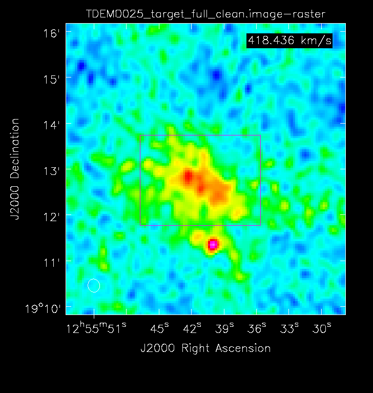
Using the viewer task, inspect your image cube TDEM0025_target_full_clean.image. As you page through the different channels, you should eventually come across some obvious HI emission within channels 2028~2062.
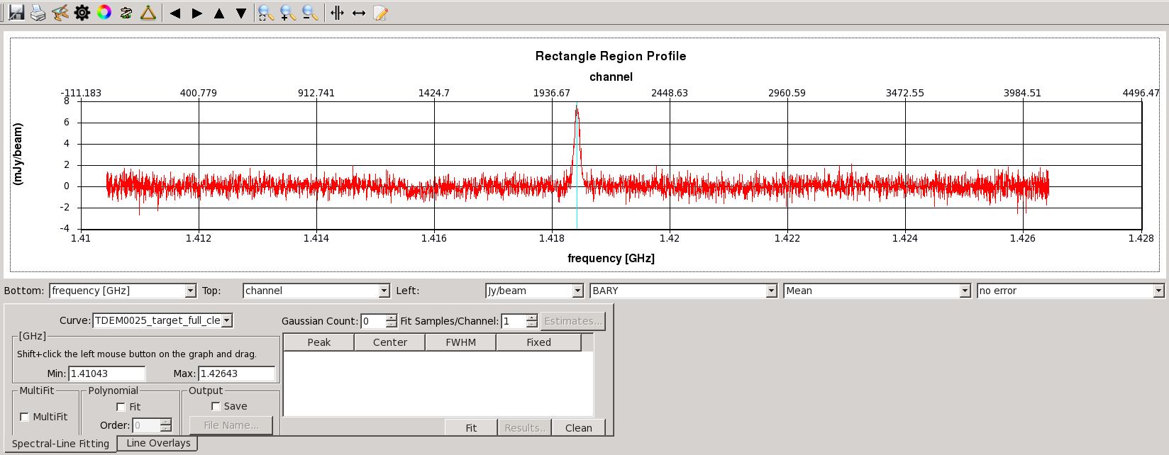
Now go to channel ~2045 (this is roughly the peak of the emission) and draw a region around the emission as shown in Figure 18. If you click on the Spectral profile ![]() button, this will generate a separate GUI which displays a spectrum of the cube data within the region you selected (Figure 19). The vertical line represents the channel within the cube that you are currently looking at. Feel free to page through channels within the viewer GUI and see how this relates to the vertical line position in the spectral profile. You may also click and drag a box, starting from the top left, to zoom in on a section of the spectrum.
button, this will generate a separate GUI which displays a spectrum of the cube data within the region you selected (Figure 19). The vertical line represents the channel within the cube that you are currently looking at. Feel free to page through channels within the viewer GUI and see how this relates to the vertical line position in the spectral profile. You may also click and drag a box, starting from the top left, to zoom in on a section of the spectrum.
As you can see, this method is prone to including continuum noise within our selected region. In the next section we will attempt to remedy this by subtracting out the continuum emission from our profile.
Step 12: Continuum Subtraction
There are three commonly used methods in CASA to subtract continuum emission, each using a different CASA task. The most precise method involves using tclean to create a model image of the continuum emission, subtracting this model from the MS using the uvsub task, and then imaging the continuum-subtracted emission in tclean. This method, while very robust, can be rather time-intensive so there are two other options.
The CASA task uvcontsub is used to subtract the continuum from a MS before imaging, and the CASA task imcontsub is used post-imaging to subtract the continuum directly from the produced image. Whereas the uvsub method requires creating a model of the continuum emission by imaging the continuum, the uvcontsub and imcontsub tasks function by estimating the continuum emission via polynomial fitting. This is inherently quicker but gives the user less control over the continuum emission selection.
Using uvsub
The CASA task uvsub provides a method for subtracting model visibilities over an entire MS. This can be useful for other cases besides continuum subtraction, like removing a bright outlier source that dominates the image. We will begin by making a copy of the TDEM0025_target_corrected.ms to serve as a backup file or beginning point for other methods of continuum subtraction.
# Psuedo-interactive CASA
!cp -r TDEM0025_target_corrected.ms TDEM0025_uvsub.ms
We then can use tclean to create a model of the continuum we wish to subtract later using the uvsub task.
# Interactive CASA
default tclean
inp
vis='TDEM0025_uvsub.ms'
imagename='TDEM0025_uvsub_contmodel'
datacolumn='data'
specmode='mfs'
cell=['3.0arcsec','3.0arcsec']
imsize=[320,320]
pblimit=-0.0001
niter=1000000
interactive=True
savemodel='modelcolumn'
inp
go
# Psuedo-interactive CASA
tclean(vis='TDEM0025_uvsub.ms', imagename='TDEM0025_uvsub_contmodel',
datacolumn='data', specmode='mfs', cell=['4.0arcsec','4.0arcsec'], imsize=[320,320], pblimit=-0.0001, niter=1000000, savemodel='modelcolumn', interactive=True)
Where:
    vis='TDEM0025_uvsub.ms'                               # the copied MS we will use for uvsub
    imagename='TDEM0025_uvsub_contmodel'                  # the name of our continuum model image
    datacolumn='data'                                     # using the data column of the copied MS
    specmode='mfs'                                        # continuum imaging with a single output image channel
    cell=['3.0arcsec','3.0arcsec']                        # cell/pixel size
    imsize=[320,320]                                      # image size in arcsec
    pblimit=-0.0001                                       # primary beam gain level cutoff
    niter=1000000                                         # arbitrarily large value to ensure niter limit is not reached and cleaning can be stopped manually
    interactive=True                                      # interactive cleaning
    savemodel='modelcolumn'                               # saves predicted model visibilities in the MODEL_DATA column of the MS
Note about iterations ~1700, also include image of mask if available. uvsub to remove continuum once satisfied
# Interactive CASA
default uvsub
inp
vis='TDEM0025_uvsub.ms'
inp
go
# Psuedo-interactive CASA
uvsub(vis='TDEM0025_uvsub.ms')
REWRITE: same steps in step 11
# Interactive CASA
default tclean
inp
vis='TDEM0025_uvsub.ms'
imagename='TDEM0025_uvsub_initial_clean'
datacolumn='data'
specmode='cube'
spw='0:3000'
niter=1
cell=['4.0arcsec','4.0arcsec']
imsize=[320,320]
nchan=1
interactive=True
inp
go
# Psuedo-interactive CASA
tclean(vis='TDEM0025_uvsub.ms', imagename='TDEM0025_uvsub_initial_clean',
datacolumn='data', specmode='cube', spw='0:3000', niter=1, cell=['4.0arcsec','4.0arcsec'], imsize=[320,320], nchan=1, interactive=True)
REWRITE: use viewer to find appropriate threshold, ~0.0028Jy
# Interactive CASA
default tclean
inp
vis='TDEM0025_uvsub.ms'
imagename='TDEM0025_uvsub_full_clean'
datacolumn='data'
specmode='cube'
niter=1000000
threshold='0.0108Jy'
cell=['3.0arcsec','3.0arcsec']
imsize=[320,320]
outframe='bary'
veltype='optical'
restfreq='1420.405752MHz'
robust=0.3
inp
go
# Psuedo-interactive CASA
tclean(vis='TDEM0025_uvsub.ms', imagename='TDEM0025_uvsub_full_clean', datacolumn='data', specmode='cube', niter=1000000, threshold='0.0108Jy',
cell=['3.0arcsec','3.0arcsec'], imsize=[320,320], outframe='bary', veltype='optical', restfreq='1420.405752MHz', robust=0.3)
REWRITE: using view
Using uvcontsub
The CASA task uvcontsub provides a method for subtracting the continuum out of the MS before imaging by performing continuum fitting and subtraction in the uv plane. This will require less steps than the uvsub method, but relies on CASA correctly fitting polynomials to the real and imaginary parts of the continuum spectrum based on the provided spectral windows and channels.
We will use a fit order of 0 which will assume that the continuum spectrum is constant. Using a fit order greater than 1 is strongly discouraged as high order polynomials can absorb line emission or vary drastically at the edges of the provide continuum range of spectral windows. In Step 11: Imaging with tclean, we found obvious HI emission within channels 2028~2062. Examining the previously generated image cube as well as its spectral profile, we will extend this range and define the HI emission channels from 2002~2093, defining our continuum-only channels as 0~2001 and 2094~4095.
# Interactive CASA
default uvcontsub
inp
vis=’TDEM0025_target_corrected.ms’
fitspw=’0:0~2001;2094~4095’
excludechans=False
solint=’int’
fitorder=0
want_cont=True
inp
go
# Psuedo-interactive CASA
uvcontsub(vis=’TDEM0025_target_corrected.ms’, fitspw=’0:0~2001;2094~4095’, excludechans=False, solint=’int’, fitorder=0, want_cont=True)
Where:

    vis='TDEM0025_target_corrected.ms'                    # the split target ms
    fitspw='0:0~2001;2094~4095'                           # the emission-free channels
    excludechans=False                                    # the defined range is the continuum
    fitorder=0                                            # polynomial order for continuum fitting
    wantcont=True                                         # will produce a continuum only measurement set as well
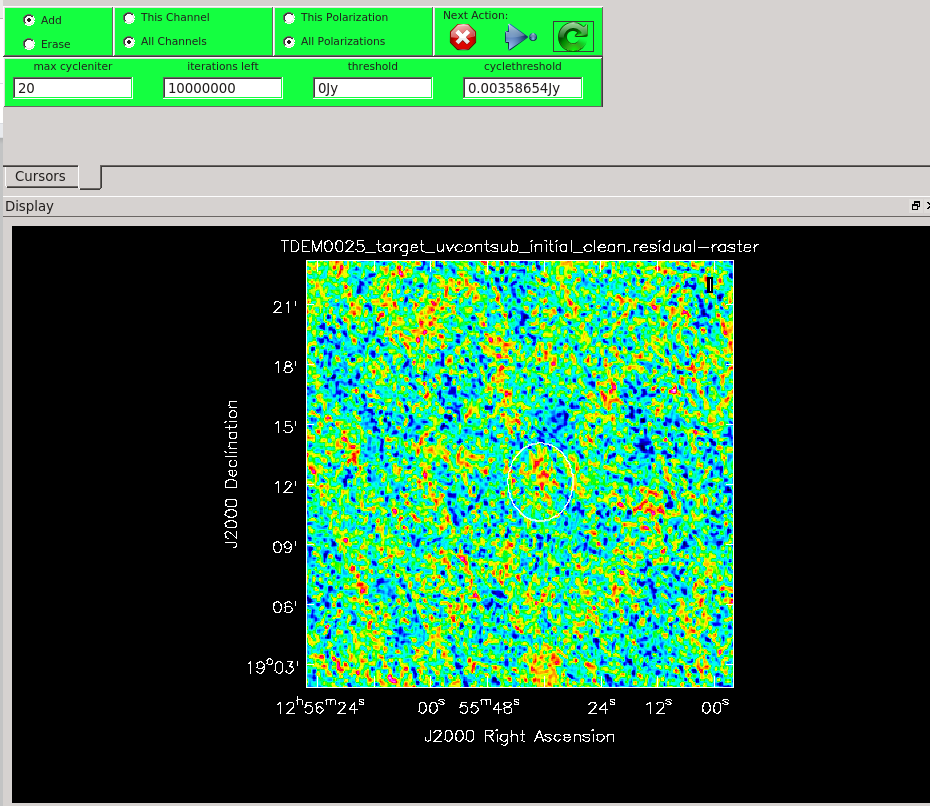
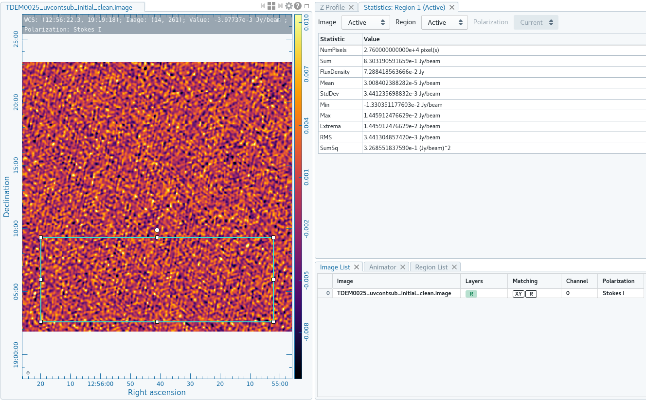
This task will produce two new measurement sets, TDEM0025_target_correct.ms.contsub and TDEM0025_target_correct.ms.cont which will contain the continuum subtracted measurement set and the isolated continuum respectively. We can now repeat the imaging process detailed in Step 11: Imaging with tclean, using TDEM0025_target_correct.ms.contsub as our visibility file to produce an image of the continuum subtracted emission. We start by cleaning a single line-free channel so we can determine the cleaning threshold to use for our full image cube, as shown in Figure ##.
# Interactive CASA
default tclean
inp
vis='TDEM0025_target_corrected.ms.contsub'
imagename='TDEM0025_target_uvcontsub_initial_clean'
datacolumn='data'
specmode='cube'
spw='0:3000'
niter=1
cell=['4.0arcsec','4.0arcsec']
imsize=[320,320]
nchan=1
interactive=True
inp
go
# Psuedo-interactive CASA
tclean(vis='TDEM0025_target_corrected.ms.contsub', imagename='TDEM0025_target_uvcontsub_initial_clean',
datacolumn='data', specmode='cube', spw='0:3000', niter=1, cell=['4.0arcsec','4.0arcsec'], imsize=[320,320], nchan=1, interactive=True)
We can once again use the viewer task to open TDEM0025_target_uvcontsub_initial_clean.image. Following the method detailed in Step 11's initial cube, we can create a rectangular region and use the Statistics tab under the Region properties to record the RMS. Here in Figure ##, our image shows an RMS of about 0.0027Jy.
As in the imaging step, we will clean all 4096 channels non-interactively using a threshold stopping criterion of approximately 4σ of the noise level (about 0.0108Jy) in tclean. Again, let the niter parameter be some arbitrarily large number to ensure the threshold is reached.
# Interactive CASA
default tclean
inp
vis='TDEM0025_target_corrected.ms.contsub'
imagename='TDEM0025_target_uvcontsub_full_clean'
datacolumn='data'
specmode='cube'
niter=1000000
threshold='0.0108Jy'
cell=['3.0arcsec','3.0arcsec']
imsize=[320,320]
outframe='bary'
veltype='optical'
restfreq='1420.405752MHz'
robust=0.3
inp
go
# Psuedo-interactive CASA
tclean(vis='TDEM0025_target_corrected.ms.contsub', imagename='TDEM0025_target_uvcontsub_full_clean', datacolumn='data', specmode='cube', niter=1000000, threshold='0.0108Jy',
cell=['3.0arcsec','3.0arcsec'], imsize=[320,320], outframe='bary', veltype='optical', restfreq='1420.405752MHz', robust=0.3)
We can again use the viewer to examine TDEM0025_target_uvcontsub_full_clean.image.
Using imcontsub
The CASA task imcontsub provides a simple method of estimating and subtracting continuum emission from an image cube. This task works similarly to uvcontsub in that it will estimate the continuum emission by fitting polynomials to a provided subset of channels. We will continue to define the continuum as channels 0~2001 and 2094~4095. We will use the TDEM0025_target_uvcontsub_full_clean image cube created in Step 11: Imaging with tclean, and also continue to use a fit order of 0 for consistency as well as the reasons stated in Using uvcontsub.
# Psuedo-interactive CASA
imcontsub(imagename=’TDEM0025_target_full_clean.image’, linefile=’TDEM0025_imcontsub.image’, contfile=’TDEM0025_imcont.image’, fitorder=0, chans=’0~2001,2094~4095’)
# Interactive CASA
default imcontsub
inp
imagename=’TDEM0025_target_full_clean.image’
linefile=’TDEM0025_imcontsub.image’
contfile=’TDEM0025_imcont.image’
fitorder=0
chans=’0~2001,2094~4095’
inp
go
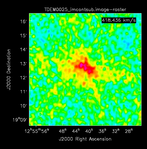
This task produces two images, TDEM0025_imcontsub.image and TDEM0025_imcont.image which will be image cubes of the continuum subtracted emission and the isolated continuum respectively.
temporary scratch room
!cp -r TDEM0025_target_corrected.ms TDEM0025_uvsub.ms
# Interactive CASA
default tclean
inp
vis=’TDEM0025_uvsub.ms’
imagename=’TDEM0025_uvsub_contmodel’
spw=’0’
imsize=[320,320]
cell=[‘3.0arcsec’,’3.0arcsec’]
specmode=’mfs’
pblimit=-0.0001
niter=100000
interactive=True
savemodel=’modelcolumn’
inp
go
# Psuedo-interactive CASA
tclean(vis='TDEM0025_uvsub.ms', imagename=’TDEM0025_uvsub_contmodel’, spw=’0’, imsize=[320,320], cell=[‘3.0arcsec’,’3.0arcsec’], specmode=’mfs’, pblimit=-0.0001, niter=100000, interactive=True, savemodel=’modelcolumn’)