VLA Self-calibration Tutorial-CASA5.7.0

This page is currently under construction.

Introduction

This CASA guide describes the basics of the self-calibration process and in particular how to choose parameters to achieve the best result. Even after the initial calibration of the dataset using the amplitude calibrator and the phase calibrator, there are likely to be residual phase and/or amplitude errors in the data. Self-calibration is the process of using an existing model, often constructed from imaging the data itself, to reduce the remaining phase and amplitude errors in your image.

The dataset that will be used for this CASA tutorial is an observation of a massive galaxy cluster at z~1 which was taken with the goal to determine the morphology of the radio sources within the cluster.

Data for this Tutorial

Observation Details

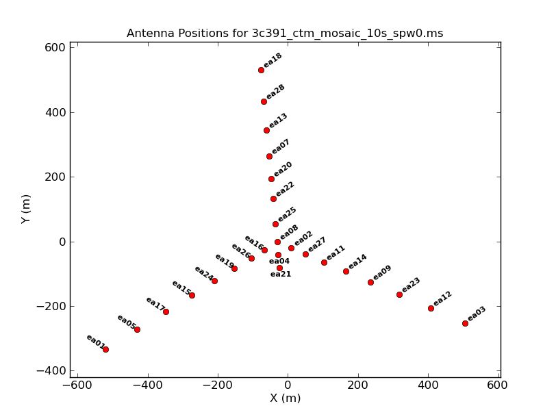
Once CASA is up and running in the directory containing the data, then start your data reduction by getting some basic information about the data. The task listobs can be used to get a listing of the individual scans comprising the observation, the frequency setup, source list, and antenna locations.

# in CASA
listobs(vis='MOO_1506+5136_Cband.ms')

================================================================================
           MeasurementSet Name:  /filepath/     MS Version 2
================================================================================
   Observer: Prof. Anthony H. Gonzalez     Project: uid://evla/pdb/34052589  
Observation: EVLA
Data records: 5290272       Total elapsed time = 2853 seconds
   Observed from   13-Oct-2017/20:40:09.0   to   13-Oct-2017/21:27:42.0 (UTC)

Initial Imaging

First, we want to make an initial image which showcases why we need self-calibration in this case.

We split off the calibrated target field data, meaning that the visibilities of the target source to get copied from the CORRECTED_DATA column to the DATA column of a new measurement set. This is convenient for further processing.

# in CASA
split(vis='MOO_1506+5236_Cband.ms',datacolumn='corrected',field='MOO_1506+3156',outputvis='obj.ms')

Now, we can make a preliminary clean image before rounds of self-calibration to use as a reference.

# in CASA
tclean(vis='obj.ms',imagename='obj.first_clean.image',imsize=750,cell='0.24arcsec',niter=1000,interactive=True)

• imsize=750:
• cell='0.24arcsec':
• niter=1000: Set a relatively large number of iterations as a starting point.
• interactive=True: Doing this interactively allows us to get a feel for the source structure and interactively place the mask.

Figure 1: plotants figure

Self-Calibration Process Outline

Each "round" of self-calibration follows a general procedure:

1. Conservatively clean target. Using interactive clean, only include the pixels that you are absolutely certain are real emission as this will be the basis of the model for calibration.
2. Use gaincal with a particular solution interval to calculate a table of solutions.
3. Check the solutions using plotcal.
4. Determine if the solutions should be applied (or if it is time to stop). Is there structure to the solutions?
5. Use applycal to apply the table of solutions to the data.
6. Use split to make the calibrated data with the applied solutions, the new data (the starting point for the next round of self-cal).
7. Start the next round of self-cal.

This guide will cover:

• How to do the self-calibration process in general.
• How to determine optimal selfcal parameters (e.g. solution interval).
• When to stop self-cal.

First Round of Self-Calibration

For this first round of self-cal, we will explore various parameters in order to settle on the optimal parameters.