EVLA spectral line IRC10216
Overview
Summer school data on IRC+10216. One subband was observed in each of two basebands, the subbands were centered on the HC3N and SiS lines near 36 GHz. Data were loaded with importevla, zero and shadowed data were flagged. Then the data were split averaging to 10 seconds and selecting only antennas with a Ka-band receiver, and the spws with Ka-band data.
Information from observing log:
There are no Ka-band receivers on ea11, ea13, ea14, ea16, ea17, ea18, ea26
Antennas ea10, ea06 are out of the array
Antenna ea12 is newly back
The pointing is often bad on ea15
Antennas ea10, ea12, ea22 do not have good baseline positions
Initial Flagging and Inspection
# In CASA
listobs(vis='day2_TDEM0003_10s_norx')
Fields: 4
  ID   Code Name         RA            Decl           Epoch   SrcId nVis
  2    D    J0954+1743   09:54:56.8236 +17.43.31.2224 J2000   2     65326
  3    NONE IRC+10216    09:47:57.3820 +13.16.40.6600 J2000   3     208242
  5    F    J1229+0203   12:29:06.6997 +02.03.08.5982 J2000   5     10836
  7    E    J1331+3030   13:31:08.2880 +30.30.32.9589 J2000   7     5814
   (nVis = Total number of time/baseline visibilities per field)
Spectral Windows:  (2 unique spectral windows and 1 unique polarization setups)
  SpwID  #Chans Frame Ch1(MHz)    ChanWid(kHz)TotBW(kHz)  Ref(MHz)    Corrs
  0          64 TOPO  36387.2295  125         8000        36387.2295  RR  RL  LR  LL
  1          64 TOPO  36304.542   125         8000        36304.542   RR  RL  LR  LL
Sources: 10
  ID   Name         SpwId RestFreq(MHz)  SysVel(km/s)
  0    J1008+0730   0     0.03639232     -0.026
  0    J1008+0730   1     0.03639232     -0.026
  2    J0954+1743   0     0.03639232     -0.026
  2    J0954+1743   1     0.03639232     -0.026
  3    IRC+10216    0     0.03639232     -0.026
  3    IRC+10216    1     0.03639232     -0.026
  5    J1229+0203   0     0.03639232     -0.026
  5    J1229+0203   1     0.03639232     -0.026
  7    J1331+3030   0     0.03639232     -0.026
  7    J1331+3030   1     0.03639232     -0.026
Antennas: 19:
  ID   Name  Station   Diam.    Long.         Lat.
  0    ea01  W09       25.0 m   -107.37.25.2  +33.53.51.0
  1    ea02  E02       25.0 m   -107.37.04.4  +33.54.01.1
  2    ea03  E09       25.0 m   -107.36.45.1  +33.53.53.6
  3    ea04  W01       25.0 m   -107.37.05.9  +33.54.00.5
  4    ea05  W08       25.0 m   -107.37.21.6  +33.53.53.0
  5    ea07  N06       25.0 m   -107.37.06.9  +33.54.10.3
  6    ea08  N01       25.0 m   -107.37.06.0  +33.54.01.8
  7    ea09  E06       25.0 m   -107.36.55.6  +33.53.57.7
  8    ea12  E08       25.0 m   -107.36.48.9  +33.53.55.1
  9    ea15  W06       25.0 m   -107.37.15.6  +33.53.56.4
  10   ea19  W04       25.0 m   -107.37.10.8  +33.53.59.1
  11   ea20  N05       25.0 m   -107.37.06.7  +33.54.08.0
  12   ea21  E01       25.0 m   -107.37.05.7  +33.53.59.2
  13   ea22  N04       25.0 m   -107.37.06.5  +33.54.06.1
  14   ea23  E07       25.0 m   -107.36.52.4  +33.53.56.5
  15   ea24  W05       25.0 m   -107.37.13.0  +33.53.57.8
  16   ea25  N02       25.0 m   -107.37.06.2  +33.54.03.5
  17   ea27  E03       25.0 m   -107.37.02.8  +33.54.00.5
  18   ea28  N08       25.0 m   -107.37.07.5  +33.54.15.8
Summary of Observing Strategy
Gain Calibrator: J0954+1743 field id=2
Bandpass Calibrator: J1229+0203   field id=5
Flux Calibrator: J1331+3030 (3C286) field id=7
Target: IRC+10216  field id=3
Ka-band spws = 0,1

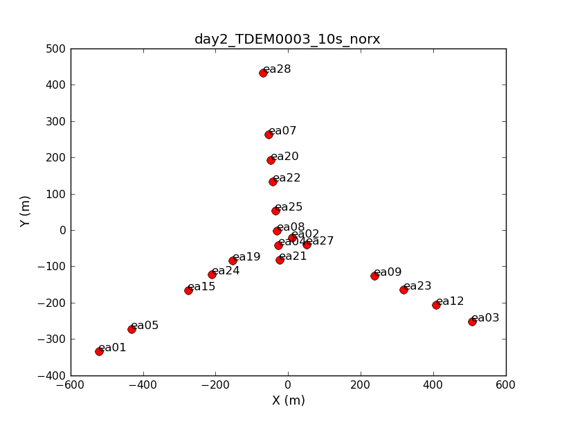
Look at a graphical plot of the antenna locations and save hardcopy in case you want it later.

# In CASA
plotants(vis='day2_TDEM0003_10s_norx',figfile='ant_locations.png')

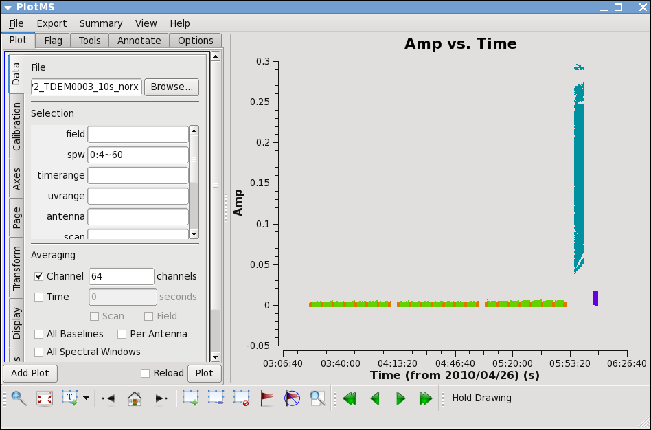
# In CASA
plotms(vis='day2_TDEM0003_10s_norx',
       xaxis='time',yaxis='amp',correlation='RR,LL',
       avgchannel='64',spw='0:4~60')
Select the "Display" tab and colorize by field.
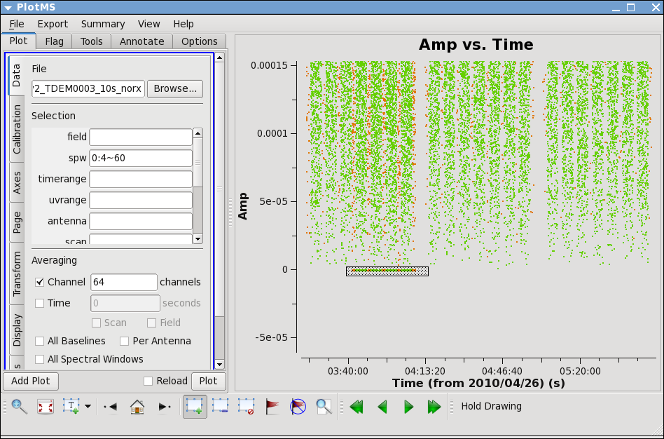
Now zoom in on the region near zero for sources J0954+1743 and IRC+10216 Look for the low values. Use the Mark and Locate buttons to see which antenna it is: ea12 Now zoom further to see the time range: 03:41:00~04:10:00
Check the other sideband by changing spw to 1:4~60. You will have to rezoom. If you have trouble click on Mark icon and then back to zoom. In spw=1, ea07 is bad from the beginning until after next pointing run: 03:21:40~04:10:00
Now try setting !ea07 in the antenna parameter, this removes ea07 from the plot allowing you to see that ea12 is also bad during the same time range as for spw 0
We can set up a flagging command to get both bad antennas for the appropriate time/spw
# In CASA
flagdata(vis='day2_TDEM0003_10s_norx',
         field=['2,3','2,3'],
         spw=['','1'],
         antenna=['ea12','ea07'],
         timerange=['03:41:00~04:10:00','03:21:40~04:10:00'])
Note because timerange is set, the field parameter is not really needed here -- the time range is limited to these fields, but flagdata will run fastest if you put as many constraints as possible.
Now remove the !ea07 from antenna and replot both spw, zooming in to be sure that all obviously low points are gone. Also zoom in and check 3C286, J1229+0203 is already obvious because it is so bright.

Lets look more closely at IRC+10216
# In CASA
plotms(vis='day2_TDEM0003_10s_norx',field='3',
       xaxis='time',yaxis='amp',correlation='RR,LL',
       avgchannel='64',spw='0~1:4~60')
Go to the "display" tab and chose colorize by spw. You can see a that there are some noisy high points. But now try
# In CASA
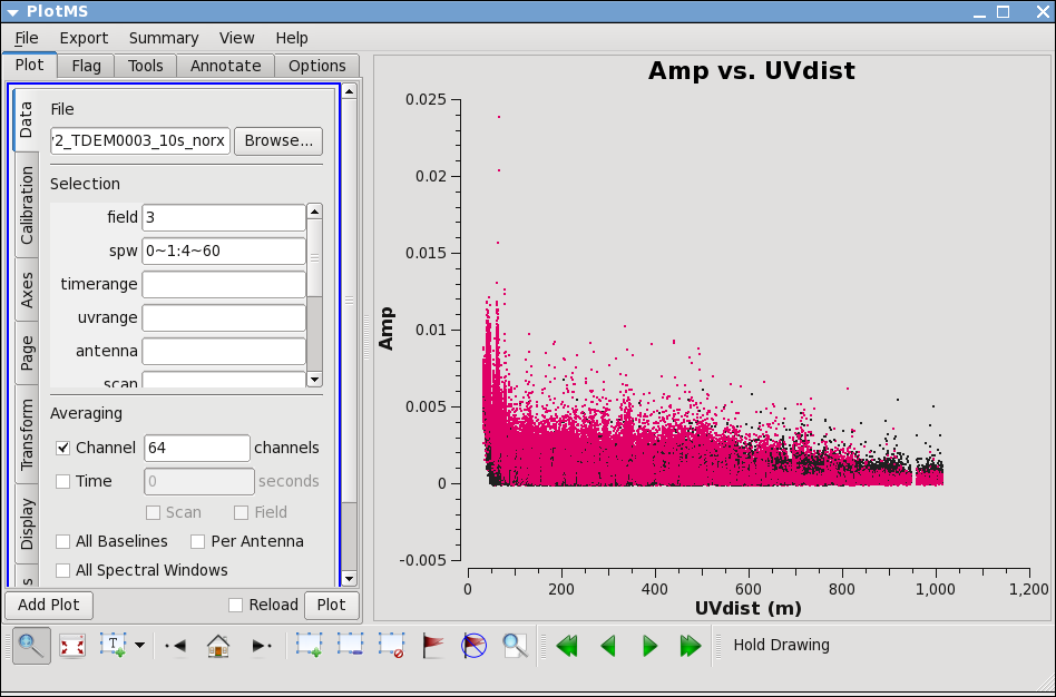
plotms(vis='day2_TDEM0003_10s_norx',field='3',
       xaxis='uvdist',yaxis='amp',correlation='RR,LL',
       avgchannel='64',spw='0~1:4~60')
Most of the high points on IRC+10216 are due to large scale emission on short baselines, but there is still some noisy stuff -- do a locate, to see that antenna ea21 looks suspicious, you can set antenna=!ea21 to see the effect of removing it. The rest of the scatter does not appear associated with a particular antenna or time. We will wait until later to decide what to do about it. If its really bad, it we won't be able to get a good calibration for it.
Set the Flux Calibrator
# In CASA
setjy(vis='day2_TDEM0003_10s_norx',field='7',spw='0',
      modimage='/usr/lib64/casapy/data/nrao/VLA/CalModels/3C286_K.im')
# In CASA
setjy(vis='day2_TDEM0003_10s_norx',field='7',spw='1',
      modimage='/usr/lib64/casapy/data/nrao/VLA/CalModels/3C286_K.im')
The logger output for spw=0 is:
setjy	J1331+3030  spwid=  0  [I=1.692, Q=0, U=0, V=0] Jy, (Perley-Taylor 99)
setjy	Using model image /usr/lib64/casapy/data/nrao/VLA/CalModels/3C286_K.im
setjy	The model image's reference pixel is 0.00188929 arcsec from J1331+3030's phase center.
setjy	Scaling model image to I=1.69182 Jy for visibility prediction.
Bandpass
Before doing the bandpass we need to inspect phase and amplitude variations with time and frequency on the bandpass calibrator to decide how best to proceed. We limit the number of antennas to make the plot easier to see. We chose ea02 as it seems like a good candidate for the reference antenna.
# In CASA
plotms(vis='day2_TDEM0003_10s_norx',field='5',
       xaxis='channel',yaxis='phase',correlation='RR',
       avgtime='1e8',spw='0:4~60',antenna='ea02&ea23')
The phase variation is modest ~10 degrees. Now expand to all antennas with ea02 and select colorize by Antenna2.
# In CASA
plotms(vis='day2_TDEM0003_10s_norx',field='5',
       xaxis='channel',yaxis='phase',correlation='RR',
       avgtime='1e8',spw='0:4~60',antenna='ea02')
Go to the "display" tab and chose colorize by antenna2. From this you can see that the phase variation across the bandpass is modest. Next check LL, and spw=1, both correlations. Also check other antennas if you like.
Now look at the phase as a function of time.
# In CASA
plotms(vis='day2_TDEM0003_10s_norx',field='5',
       xaxis='time',yaxis='phase',correlation='RR',
       avgchannel='64',spw='0:4~60',antenna='ea02&ea23')
Expand to all antennas with ea02
# In CASA
plotms(vis='day2_TDEM0003_10s_norx',field='5',
       xaxis='time',yaxis='phase',correlation='RR',
       avgchannel='64',spw='0:4~60',antenna='ea02')
You can see that the phase variations are smooth, but do vary significantly over the 5 minutes of observation -- in most cases by a few 10s of degrees. Zoom in to see this better if you want.
The conclusion from this investigation is that you need to correct the phase variations with time before solving for the bandpass to prevent decorrelation of the vector averaged bandpass solution. Since the phase variation as a function of channel is modest, you can average over several channels to increase the signal to noise of the phase vs. time solution. If the phase variation as a function of channel is larger you may need to use only a few channels to delay-based closure errors from averaging over non-bandpass corrected channels.
Since the bandpass calibrator is quite strong we do the phase-only
solution on the integration time of 10 seconds (solint='int').
# In CASA
gaincal(vis='day2_TDEM0003_10s_norx',caltable='bpphase.gcal',
        field='5',spw='0~1:20~40',
        refant='ea02',calmode='p',solint='int',minsnr=2.0)
# In CASA
plotcal(caltable='bpphase.gcal',xaxis='time',yaxis='phase',
        iteration='antenna',subplot=331)
Next we can apply this phase solution on the fly while determining
the bandpass solutions, solint='inf' will derive a one bandpass
solution for the whole J1229+0203 scan. If there had been two
observations of the bandpass calibration for example, this command
would do one bandpass for each scan, if combine= (combine='scan'
is the default).
# In CASA
bandpass(vis='day2_TDEM0003_10s_norx',caltable='bandpass.bcal',field='5',
        refant='ea02',solint='inf',solnorm=T,
# In CASA
gaintable=['bpphase.gcal'],spwmap=[[]])
This step isn't necessary from a calibration perspective, but if you want to go ahead and check the bandpass calibration on the bandpass calibrator you can run applycal here. In future we hope to plot corrected data on-the-fly without this applycal step. Later applycals will overwrite this one, so no need to worry.
# In CASA
applycal(vis='day2_TDEM0003_10s_norx',field='5',
        gaintable=['bandpass.bcal'],
        spwmap=[[]],gainfield=['5'])
# In CASA
plotcal(caltable='bandpass.bcal',xaxis='chan',yaxis='amp',
        iteration='antenna',subplot=331)
# In CASA
plotcal(caltable='bandpass.bcal',xaxis='chan',yaxis='phase',
        iteration='antenna',subplot=331)
Note that phases on ea12 look noiser than other antennas. This jitter could indicate bad pointing -- note ea12 had just come back in the array.
Gain Calibration
# In CASA
gaincal(vis='day2_TDEM0003_10s_norx',caltable='intphase.gcal',
        field='2,5,7',spw='0~1:4~60',
        refant='ea02',calmode='p',solint='int',minsnr=2.0,
        gaintable=['bandpass.bcal'],spwmap=[[]])
# In CASA
plotcal(caltable='intphase.gcal',xaxis='time',yaxis='phase',
        iteration='antenna',subplot=331)
# In CASA
gaincal(vis='day2_TDEM0003_10s_norx',caltable='scanphase.gcal',
        field='2,5,7',spw='0~1:4~60',
        refant='ea02',calmode='p',solint='inf',minsnr=2.0,
        gaintable=['bandpass.bcal'],spwmap=[[]])
# In CASA
plotcal(caltable='scanphase.gcal',xaxis='time',yaxis='phase',
        iteration='antenna',subplot=331)
# In CASA
gaincal(vis='day2_TDEM0003_10s_norx',caltable='amp.gcal',
        field='2,5,7',spw='0~1:4~60',
        refant='ea02',calmode='ap',solint='inf',minsnr=2.0,
        gaintable=['bandpass.bcal','intphase.gcal'],spwmap=[[],[]])
# In CASA
plotcal(caltable='amp.gcal',xaxis='time',yaxis='phase',
        iteration='antenna',subplot=331)
# In CASA
plotcal(caltable='amp.gcal',xaxis='time',yaxis='amp',
        iteration='antenna',subplot=331)
# In CASA
fluxscale(vis='day2_TDEM0003_10s_norx',caltable='amp.gcal',
          fluxtable='flux.cal',reference='7')
# In CASA
plotcal(caltable='flux.cal',xaxis='time',yaxis='amp',
        iteration='antenna',subplot=331)
fluxscale Flux density for J0954+1743 in SpW=0 is: 0.274144 +/- #0.00108416 (SNR = 252.862, nAnt= 18)
fluxscale Flux density for J0954+1743 in SpW=1 is: 0.280975 +/- #0.00107734 (SNR = 260.805, nAnt= 18)
fluxscale Flux density for J1229+0203 in SpW=0 is: 30.4866 +/- 0(SNR = inf, nAnt= 18)
fluxscale Flux density for J1229+0203 in SpW=1 is: 30.1742 +/- 0(SNR = inf, nAnt= 18)
# In CASA
plotms(vis='day2_TDEM0003_10s_norx',field='5',ydatacolumn='corrected',
       xaxis='time',yaxis='amp',correlation='RR,LL',
       avgchannel='64',spw='0:4~60',antenna='')
Applycal and Inspect
# In CASA
applycal(vis='day2_TDEM0003_10s_norx',field='2',
        gaintable=['bandpass.bcal','intphase.gcal','flux.cal'],
        spwmap=[[],[],[]],gainfield=['5','2','2'])
# In CASA
applycal(vis='day2_TDEM0003_10s_norx',field='5',
        gaintable=['bandpass.bcal','intphase.gcal','flux.cal'],
        spwmap=[[],[],[]],gainfield=['5','5','5'])
# In CASA
applycal(vis='day2_TDEM0003_10s_norx',field='7',
        gaintable=['bandpass.bcal','intphase.gcal','flux.cal'],
        spwmap=[[],[],[]],gainfield=['5','7','7'])
# In CASA
applycal(vis='day2_TDEM0003_10s_norx',field='3',
        gaintable=['bandpass.bcal','scanphase.gcal','flux.cal'],
        spwmap=[[],[],[]],gainfield=['5','2','2'])
Now inspect the corrected data
# In CASA
plotms(vis='day2_TDEM0003_10s_norx',field='5',ydatacolumn='corrected',
       xaxis='time',yaxis='amp',correlation='RR,LL',
       avgchannel='64',spw='0:4~60',antenna='')
This source looks good
# In CASA
plotms(vis='day2_TDEM0003_10s_norx',field='2',ydatacolumn='corrected',
       xaxis='time',yaxis='amp',correlation='RR,LL',
       avgchannel='64',spw='0:4~60',antenna='')
Here we see some problems, with high points. Do some mark regions and locate to find out which antennas, which spws. Pay special attention to antennas that shows some dubious behavior from the start.
What you find is that ea07 which we flagged spw=1 above, is also bad for the same timerange in spw=0. This was not obvious in the raw data, because spw=0 was adjusted by a gain attenuator, while spw=1 wasn't. So a lack of power in spw=1 will look like very low amplitudes -- not so after the adjustment made to spw=0.
ea12 needs to be flagged completely its just a bit noisy all around.
ea23 is pretty noisy during the first scans between intial and second pointing.
Because the target has resolved structure, its best to look at it as a function of uvdistance.
# In CASA
plotms(vis='day2_TDEM0003_10s_norx',field='3',ydatacolumn='corrected',
       xaxis='uvdist',yaxis='amp',correlation='RR,LL',
       avgchannel='64',spw='0:4~60',antenna='')
in "display" tab chose colorize by antenna2, here you will see that the spikes are caused by a single antenna. Use, zoom, mark, and locate to see which one. Also look at spw=1.
Turns out to be ea28, to confirm, replot with antenna=!ea28, and
# In CASA
plotms(vis='day2_TDEM0003_10s_norx',field='3',ydatacolumn='corrected',
       xaxis='uvdist',yaxis='amp',correlation='RR,LL',
       avgchannel='64',spw='0:4~60',antenna='ea28')
Its got issues until 2/3 through. Plot another distant antenna to compare. We will go ahead and flag it all, since its hanging far out on the north arm by itself.
These data need to be flagged and then all the calibration steps run again.
# In CASA
flagdata(vis='day2_TDEM0003_10s_norx',
         field=['',''],
         spw=['',''],
         antenna=['ea12,ea28','ea07,ea23'],
         timerange=['','03:21:40~04:10:00'])
Redo Calibration after more Flagging
# In CASA
gaincal(vis='day2_TDEM0003_10s_norx',caltable='bpphase_redo.gcal',
        field='5',spw='0~1:20~40',
        refant='ea02',calmode='p',solint='int',minsnr=2.0)
# In CASA
bandpass(vis='day2_TDEM0003_10s_norx',caltable='bandpass_redo.bcal',
        field='5',
        refant='ea02',solint='inf',solnorm=T,
        gaintable=['bpphase_redo.gcal'],spwmap=[[]])
# In CASA
gaincal(vis='day2_TDEM0003_10s_norx',caltable='intphase_redo.gcal',
        field='2,5,7',spw='0~1:4~60',
        refant='ea02',calmode='p',solint='int',minsnr=2.0,
        gaintable=['bandpass_redo.bcal'],spwmap=[[]])
# In CASA
gaincal(vis='day2_TDEM0003_10s_norx',caltable='scanphase_redo.gcal',
        field='2,5,7',spw='0~1:4~60',
        refant='ea02',calmode='p',solint='inf',minsnr=2.0,
        gaintable=['bandpass_redo.bcal'],spwmap=[[]])
# In CASA
gaincal(vis='day2_TDEM0003_10s_norx',caltable='amp_redo.gcal',
        field='2,5,7',spw='0~1:4~60',
        refant='ea02',calmode='ap',solint='inf',minsnr=2.0,
        gaintable=['bandpass_redo.bcal','intphase_redo.gcal'],
        spwmap=[[],[]])
# In CASA
fluxscale(vis='day2_TDEM0003_10s_norx',caltable='amp_redo.gcal',
          fluxtable='flux_redo.cal',reference='7')
fluxscale Flux density for J0954+1743 in SpW=0 is: 0.274097 +/- 0.00110645 (SNR = 247.726, nAnt= 18)
fluxscale Flux density for J0954+1743 in SpW=1 is: 0.281065 +/- 0.00107598 (SNR = 261.217, nAnt= 18)
fluxscale Flux density for J1229+0203 in SpW=0 is: 30.488 +/- 0 (SNR = inf, nAnt= 18)
fluxscale Flux density for J1229+0203 in SpW=1 is: 30.1777 +/- 0 (SNR = inf, nAnt= 18)
# In CASA
applycal(vis='day2_TDEM0003_10s_norx',field='2',
        gaintable=['bandpass_redo.bcal','intphase_redo.gcal','flux_redo.cal'],
        spwmap=[[],[],[]],gainfield=['5','2','2'])
# In CASA
applycal(vis='day2_TDEM0003_10s_norx',field='5',
        gaintable=['bandpass_redo.bcal','intphase_redo.gcal','flux_redo.cal'],
        spwmap=[[],[],[]],gainfield=['5','5','5'])
# In CASA
applycal(vis='day2_TDEM0003_10s_norx',field='7',
        gaintable=['bandpass_redo.bcal','intphase_redo.gcal','flux_redo.cal'],
        spwmap=[[],[],[]],gainfield=['5','7','7'])
# In CASA
applycal(vis='day2_TDEM0003_10s_norx',field='3',
        gaintable=['bandpass_redo.bcal','scanphase_redo.gcal','flux_redo.cal'],
        spwmap=[[],[],[]],gainfield=['5','2','2'])
# In CASA
plotms(vis='day2_TDEM0003_10s_norx',field='2',ydatacolumn='corrected',
       xaxis='time',yaxis='amp',correlation='RR,LL',
       avgchannel='64',spw='0:4~60',antenna='')
# In CASA
plotms(vis='day2_TDEM0003_10s_norx',field='3',ydatacolumn='corrected',
       xaxis='time',yaxis='amp',correlation='RR,LL',
       avgchannel='64',spw='0:4~60',antenna='')
Split
# In CASA
split(vis='day2_TDEM0003_10s_norx',outputvis='day2_J0954',
      field='2')
# In CASA
split(vis='day2_TDEM0003_10s_norx',outputvis='day2_IRC10216',
      field='3')
# In CASA
split(vis='day2_TDEM0003_10s_norx',outputvis='day2_3C286',
      field='7')
Clean
# In CASA
clean(vis='day2_IRC10216',imagename='day2_IRC10216_spw1.cube_r0.5',
      imagermode='csclean',
      imsize=300,cell=['0.4arcsec'],spw='1:5~58',
      mode='velocity',interpolation='linear',
      restfreq='36.30963GHz',outframe='LSRK',
      weighting='briggs',robust=0.5,
      mask='HC3N_r0.5.mask',
      interactive=F,threshold='3.0mJy',niter=100000)
# In CASA
clean(vis='day2_IRC10216',imagename='day2_IRC10216_spw0.cube_r0.5',
      imagermode='csclean',
      imsize=300,cell=['0.4arcsec'],spw='0:5~58',
      mode='velocity',interpolation='linear',
      restfreq='36.39232GHz',outframe='LSRK',
      weighting='briggs',robust=0.5,
      mask='HC3N_r0.5.mask',
      interactive=F,threshold='3.0mJy',niter=100000)
# In CASA
clean(vis='day2_IRC10216',imagename='day2_IRC10216_spw0.cube_r0.5_mulit',
      imagermode='',
      imsize=300,cell=['0.4arcsec'],spw='0:5~58',
      mode='velocity',interpolation='linear',
      restfreq='36.39232GHz',outframe='LSRK',
      weighting='briggs',robust=0.5,
      mask='HC3N_r0.5.mask',
      multiscale = [0,25,50,75],
      interactive=F,threshold='3.0mJy',niter=10000)