Sunspot Band6 SingleDish for CASA 5.1

Overview

This portion of the Sunspot Band6 CASA Guide for CASA 5.1 will cover the calibration and imaging of the data obtained with the TP array.

From next, we will show all commands for the calibration and be creating the map of a full Sun with Band6.

Import the data and split into the files for each antenna

We assume that you already complete the calibration of the visibility data along the Sunspot Band6 Calibration for CASA 5.1, and you are working in the directory ‘Sunspot_Band6_UncalibratedData’. After starting CASA, we start by defining the directory name of the ASDM and Measurement set for the calibration.

#In Casa
sduid ='uid___A002_Xae00c5_X2e6b'
sdmsd = sduid + '.ms'
sdmsc = sdmsd + '.split.cal'
ant='PM3'

In the tutorial, we will use the data obtained with the PM03 antenna.

Before we can proceed to the calibration, we will need to convert those data to the CASA MS format. This is done simply with the task importasdm.

#In Casa
importasdm(asdm=sduid,with_pointing_correction=True, verbose=True,vis=sdmsd,overwrite=True)

The usual first step is then to get some basic information about the data.

#In Casa
listobs(sdmsd, listfile = sduid + '.listobs')
aU.getTPSampling(vis = sdmsd, showplot = True, plotfile = sduid+'.sampling.png')

Calibration

In the observation, the atmospheric calibration was done before the fast-scanning of the Sun. We use the calibration date to apply the solar data using the option ‘ps, tsys, apply’ for the ‘calmode’.

#In Casa
sdcal(infile=sdmsd, calmode = 'ps,tsys,apply', spw='0,1,2,3')
split(vis = sdmsd, spw = '0,1,2,3', outputvis = admsc, scan = '6', datacolumn = 'corrected', keepflags = True)

Unlike non-solar single-dish observations, the flux calibrator is not observed in solar single-dish observations in Cycle 4. Therefore, we have to calibrate the data using a correction factor which includes various antenna efficiencies of the PM antenna.

Based on the commissioning observations, the average correction factor of the PM antennas with Band6 is 0.862, which enables us to calibrate the observed antenna temperature to the absolute brightness temperature. We will calibrate using the value, as follows.

#In Casa
gencal(vis=sdmsc,caltable=sduid+'.cal.eff.tbl', caltype='amp', spw='',parameter=[sqrt(0.862)])
applycal(vis=sdmsc, gaintable=sduid+'.cal.eff.tbl')

Caution: The correction factor in this document is written in White et al. (2017)

Imaging

<figure id="fullsun">

<xr id="fullsun" nolink/> The full-sun image with Band6

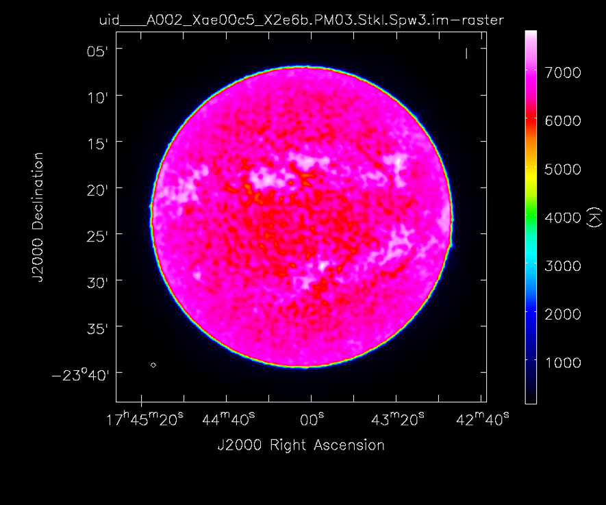
</figure> To create the full sun map, we use the data of the spectrum window #3 obtained with the PM03 antenna. The command for the process is as follows.

#In Casa
sd_img = sdmsd + '.'+ant+'.Sun_sci.spw3_248000MHz.I.sd.TP.2D.cont'
sdimaging(infiles = sdmsc, spw = '3', antenna =ant, field='1', nchan = 1, cell = ['3.0arcsec','3.0arcsec'], outfile = sd_img, imsize=[800,800], gridfunction = 'SF', convsupport = 6, intent ='*ON_SOURCE*', stokes = 'I', ephemsrcname = 'sun')

After finishing the process successfully, you can see the full-sun image as shown in <xr id="fullsun" />. When you carry out the imaging of Band3 data, we recommend the following parameters for the sdimaging task.

#In Casa
sdimaging(infiles = sdmsc, spw = '3', antenna =ant, field='1', nchan = 1, cell = ['6.0arcsec','6.0arcsec'], outfile = sd_img, imsize=[400,400], gridfunction = 'SF', convsupport = 6, intent ='*ON_SOURCE*', stokes = 'I', ephemsrcname = 'sun')

Calibration (re-scaling) after Imaging

White et al. (2017) recommended that the standard ALMA single-dish image products be scaled to match their best determination of quiet-Sun temperatures at disk center (specifically, 5900 K averaged over an 80″-square region centered on the apparent disk center at Band 6, and 7300 K averaged over a 120″-square region centered on the apparent disk center at Band 3, with uncertainties of about 100 K). For the re-scaling, the following commands are executed.

#In Casa
res = imstat(sd_img, region='circle[[400pix,400pix],80pix]')  
immath(imagename=sd_img, expr = 'IM0*'+str(5900./res['mean'][0]), outfile = sd_img+'.rescl')

Note: The reference full-sun image included in the SV data (Sunspot_Band6_ReferenceImages.tgz) were not applied the re-scaling because the SV data were released before publishing White et al. (2017). When you use the full-sun image of the SV data for your studies, you should be done the re-scaling process. While, The archive data obtained in Cycles were applied the re-scaling process.