Self-Calibration Template CASA 6.1.1
This guide continues with products created in Image_Continuum. All imaging parameters are set in the previous guide. You will need calibrated_final_cont.ms to proceed.
Self-Calibration on the Continuum (optional)
This step of imaging is optional and can be attempted in cases where the expected rms is not reached on the continuum or the line data or to improve signal to noise. Self-calibration solutions can only be determined when a source exhibits a strong continuum emission, preferably near the phase center. With this being said, self-calibration should not be performed on data sets with poor uv coverage but can be performed on “partial” data sets (like ACA _TC datasets). It is not recommended on projects that are non-detections or contain weak sources.
For a more detailed explanation of self-calibration, please see Ed Fomalont and Jeff Mangum’s Best Practices for Self-Calibration of Spectral Line Image Cubes Editing Note: this is an internal to NRAO link
Begin by declaring your ms and continuum image name. calibrated_final_cont.ms was created in the previous part of this guide, Image_Continuum.
# in CASA
contvis = 'calibrated_final_cont.ms'
contimagename = 'calibrated_final_cont'
Next, choose a reference antenna that is in the array by using the tasks plotants or listobs/vishead. For data sets with multiple executions, you will want to choose an antenna that is present in all of the executions, which can be found by using the task [au.commonAntennas]. You should use the same reference antenna that was used during calibration. For pipeline reductions, this can be found in the stage hif_refant. For manual reductions, the reference antenna will be stated near the top of *.ms.scriptForCalibration.py.
# in CASA
refant = 'DV09' # pick a reference antenna.
You will need to map the self-calibration solutions to individual spectral windows. This is generally an array of n zeros, where n is the number of spectral windows for the ms. This is the case because spwcombine is used in gaincal, which combines all solutions to a single spectral window numbered 0. By setting an array of n zeros we are applying the solution to each spectral window within the ms.
In the example below, we will apply the solutions to spws 0, 1 and 2.
# in CASA
spwmap = [0,0,0] # change to an array of n zeros
Save all of the initial flags in case the final self-calibration solution still doesn’t meet your expectations. The task applycal will flag data that does not have solutions.
# in CASA
flagmanager(vis=contvis,mode='save',versionname='before_selfcal',merge='replace')
In the case of running self-calibration more than once, you will need to remove any models that could be left in the image header; which can be accomplished by using the delmod task as well as the clearcal task (which will need to be uncommented).
# in CASA
# delmod(vis=contvis,field=field,otf=True)
# clearcal(vis=contvis)
You then begin the process of shallowly cleaning your continuum. Once the parameters for cleaning are set, and clean is run interactively, the next step is to calibrate antenna-based gains as a function of time (using gaincal) and apply solutions prior to the next cleaning. With each additional clean, the time iterations will get shorter. At this point you should clean until satisfied with the end result.
# in CASA
# shallow clean on the continuum

for ext in ['.flux','.image','.mask','.model','.pbcor','.psf','.residual','.flux.pbcoverage']:
    rmtables(contimagename + '_p0'+ ext)

clean(vis=contvis,
      imagename=contimagename + '_p0',
      field=field,
#      phasecenter=phasecenter, # uncomment if mosaic.
      mode='mfs',
      psfmode='clark',
      imsize = imsize,
      cell= cell,
      weighting = weighting,
      robust=robust,
      niter=niter,
      threshold=threshold,
      interactive=True,
      usescratch=True, # needed for 4.3 and 4.4 (and maybe 4.5)
      imagermode=imagermode)

# Note number of iterations performed.

# per scan solution
rmtables('pcal1')
gaincal(vis=contvis,
        caltable='pcal1',
        field=field,
        gaintype='T',
        refant=refant,
        calmode='p',
        combine='spw',
        solint='inf',
        minsnr=3.0,
        minblperant=6)
You may see messages about failed solutions when running gaincal. Any data that does not have solutions in the calibration table will be flagged when the calibration is applied to the ms. If too much data is flagged, the sensitivity will decrease. Look for messages in the logger about the success of the calculations. The text below shows the expected/attempted/succeeded numbers in the logger window. It is not a problem to have a few failed solutions, but be cautious if it seems many are failing. Note that you will only see successful calculations for spw 0.
Calibration solve statistics per spw: (expected/attempted/succeeded):
   Spw 0: 235/235/235
   Spw 1: 235/235/235
   Spw 2: 235/235/235
<figure id="Plotcal_image.png">

</figure> The minimum snr (minsnr) and minimum baseline per antenna (minblperant) parameters can be decreased to increase the number of solutions found.
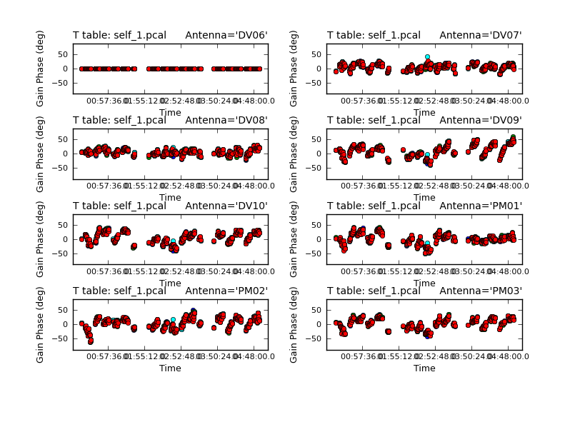
You should also check the solutions (above) that were obtained using plotcal.
In CASA
# Check the solution
plotcal(caltable='pcal1',
        xaxis='time',
        yaxis='phase',
        timerange='',
        iteration='antenna',
        subplot=421,
        plotrange=[0,0,-180,180])
If you are satisfied with the solutions, apply them to the ms and clean the new visibilities. <figure id="Pcal1.png">

</figure>
# in CASA
# apply the calibration to the data for next round of imaging
applycal(vis=contvis,
         field=field,
         spwmap=spwmap,
         gaintable=['pcal1'],
         gainfield='',
         calwt=False,
         flagbackup=False,
         interp='linearperobs')

# clean deeper
for ext in ['.flux','.image','.mask','.model','.pbcor','.psf','.residual','.flux.pbcoverage']:
    rmtables(contimagename + '_p1'+ ext)

clean(vis=contvis,
      field=field,
#      phasecenter=phasecenter, # uncomment if mosaic.
      imagename=contimagename + '_p1',
      mode='mfs',
      psfmode='clark',
      imsize = imsize,
      cell= cell,
      weighting = weighting,
      robust=robust,
      niter=niter,
      threshold=threshold,
      interactive=True,
      usescratch=True, # needed for 4.3 and 4.4 (and maybe 4.5)
      imagermode=imagermode)

# Note number of iterations performed.
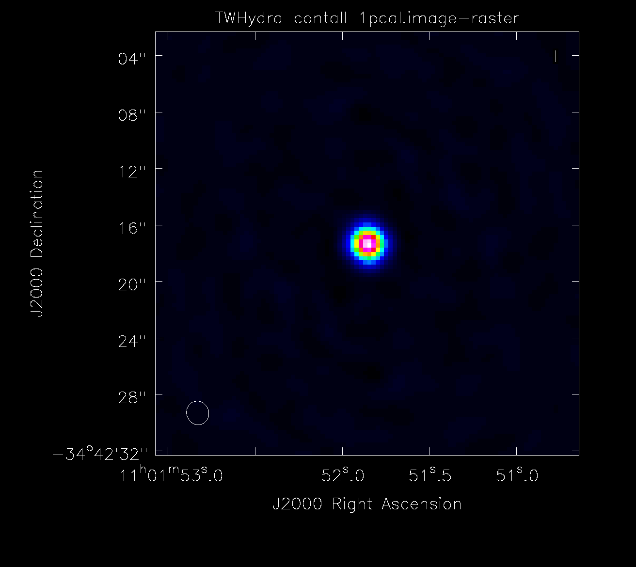
Inspect the new image in the viewer to see if the first iteration of self-cal worked. Find and compare the new RMS, beam size, and dynamic range of the image to the calibrated_final_cont_p0.image. If the RMS noise increased, do not proceed with the self-calibration. You may try changing the minsnr and minblperant parameters in the gaincal call above to find more solutions. If you are unable to improve the image using self-calibration, undo the self-calibration and skip to the continuum subtraction section of this guide. If the RMS noise and dynamic range improved, proceed with self-calibration below. The next gaincal call uses a shorter solution interval (solint). Continue on with the self-calibration as long as the image statistics continue to improve.
# in CASA
# shorter solution
rmtables('pcal2')
gaincal(vis=contvis,
        field=field,
        caltable='pcal2',
        gaintype='T',
        refant=refant,
        calmode='p',
        combine='spw',
        solint='30.25s', # solint=30.25s gets you five 12m integrations, while solint=50.5s gets you five 7m integration
        minsnr=3.0,
        minblperant=6)

# Check the solution
plotcal(caltable='pcal2',
        xaxis='time',
        yaxis='phase',
        timerange='',
        iteration='antenna',
        subplot=421,
        plotrange=[0,0,-180,180])

# apply the calibration to the data for next round of imaging
applycal(vis=contvis,
         spwmap=spwmap,
         field=field,
         gaintable=['pcal2'],
         gainfield='',
         calwt=False,
         flagbackup=False,
         interp='linearperobs')

# clean deeper
for ext in ['.flux','.image','.mask','.model','.pbcor','.psf','.residual','.flux.pbcoverage']:
    rmtables(contimagename + '_p2'+ ext)

clean(vis=contvis,
      imagename=contimagename + '_p2',
      field=field,
#      phasecenter=phasecenter, # uncomment if mosaic.
      mode='mfs',
      psfmode='clark',
      imsize = imsize,
      cell= cell,
      weighting = weighting,
      robust=robust,
      niter=niter,
      threshold=threshold,
      interactive=True,
      usescratch=True, # needed for 4.3 and 4.4 (and maybe 4.5)
      imagermode=imagermode)

# Note number of iterations performed.

# shorter solution
rmtables('pcal3')
gaincal(vis=contvis,
        field=field,
        caltable='pcal3',
        gaintype='T',
        refant=refant,
        calmode='p',
        combine='spw',
        solint='int',
        minsnr=3.0,
        minblperant=6)

# Check the solution
plotcal(caltable='pcal3',
        xaxis='time',
        yaxis='phase',
        timerange='',
        iteration='antenna',
        subplot=421,
        plotrange=[0,0,-180,180])

# apply the calibration to the data for next round of imaging
applycal(vis=contvis,
         spwmap=spwmap,
         field=field,
         gaintable=['pcal3'],
         gainfield='',
         calwt=False,
         flagbackup=False,
         interp='linearperobs')

for ext in ['.flux','.image','.mask','.model','.pbcor','.psf','.residual','.flux.pbcoverage']:
    rmtables(contimagename + '_p3'+ ext)

clean(vis=contvis,
      imagename=contimagename + '_p3',
      field=field,
#      phasecenter=phasecenter, # uncomment if mosaic.
      mode='mfs',
      psfmode='clark',
      imsize = imsize,
      cell= cell,
      weighting = weighting,
      robust=robust,
      niter=niter,
      threshold=threshold,
      interactive=True,
      usescratch=True, # needed for 4.3 and 4.4 (and maybe 4.5)
      imagermode=imagermode)

# Note number of iterations performed.
<figure id="Apcal.png">

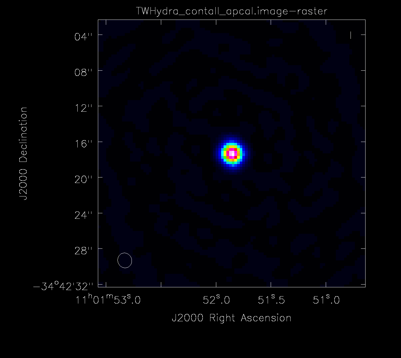
</figure> The next section performs an amplitude calibration. While the phase calibration involved iterating with different solution intervals, the amplitude self-calibration will only use an infinite solution interval.
# in CASA
rmtables('apcal')
gaincal(vis=contvis,
        field=field,
        caltable='apcal',
        gaintype='T',
        refant=refant,
        calmode='ap',
        combine='spw',
        solint='inf',
        minsnr=3.0,
        minblperant=6,
#        uvrange='>50m', # may need to use to exclude extended emission
        gaintable='pcal3',
        spwmap=spwmap,
        solnorm=True)

plotcal(caltable='apcal',
        xaxis='time',
        yaxis='amp',
        timerange='',
        iteration='antenna',
        subplot=421,
        plotrange=[0,0,0.2,1.8])

applycal(vis=contvis,
         spwmap=[spwmap,spwmap], # select which spws to apply the solutions for each table
         field=field,
         gaintable=['pcal3','apcal'],
         gainfield='',
         calwt=False,
         flagbackup=False,
         interp='linearperobs')

# Make amplitude and phase self-calibrated image.
for ext in ['.flux','.image','.mask','.model','.pbcor','.psf','.residual','.flux.pbcoverage']:
    rmtables(contimagename + '_ap'+ ext)

clean(vis=contvis,
      imagename=contimagename + '_ap',
      field=field,
 #      phasecenter=phasecenter, # uncomment if mosaic.
      mode='mfs',
      psfmode='clark',
      imsize = imsize,
      cell= cell,
      weighting = weighting,
      robust=robust,
      niter=niter,
      threshold=threshold,
      interactive=True,
      usescratch=True, # needed for 4.3 and 4.4 (and maybe 4.5)
      imagermode=imagermode)
Compare all of the images produced during self-calibration. Only apply solutions that continue to improve the image statistics.
The results of the self-cal should be split out via the split command and saved as a *.selfcal file.
# in CASA
split(vis=contvis,
outputvis=contvis+'.selfcal', datacolumn='corrected')
If you are unhappy with the self-calibration, use the clearcal task and restore the original flags to return your ms to it’s original pre-self-cal state.
# in CASA
# uncomment the following to revert to pre self-cal ms
# flagmanager(vis=contvis, mode='restore',versionname='before_selfcal')
# clearcal(contvis)
# delmod(contvis,field=field,otf=True)
You will subtract the continuum and apply the self-calibration results to the line data on the next page, Image_Line.