VLA CASA Flagging-CASA4.7.0
- This CASA guide is designed for CASA 4.7.0
- Printing Disclaimer: When printing, CASA commands in this guide may be cropped, depending on your web browser text size and printer settings.
Overview
This CASA guide covers online data flagging, shadowing, zero-clipping, and quacking. It also covers auto-flagging RFI (Radio Frequency Interference) via TFCrop (Time-Frequency Crop) and rflag.
We will be utilizing data, taken with the Karl G. Jansky Very Large Array, of G055.7+3.4., which is a supernova remnant. The data were taken on August 23, 2010 in the first D-configuration for which the new wideband capabilities of the WIDAR (Wideband Interferometric Digital ARchitecture) correlator were available. The 8 hour long session includes all available 1 GHz of bandwidth in L-band, from 1-2 GHz in frequency.
The guide will often reference the CASA cookbook which is available online and can be downloaded as a pdf.
Obtaining the Data
A copy of the data can be downloaded from http://casa.nrao.edu/Data/EVLA/SNRG55/SNR_G55_10s.tar.gz (5.0 GB). These data are already in CASA Measurement Set (MS) format and were prepared specifically for this guide.
The following explains how the data were processed as it has implications for later flagging steps. Note that commands with a grey background do not need to be run in CASA.
The data were first loaded from the NRAO archive. On the archive search form, specify Archive File ID to be AB1345_sb1800808_1.55431.004049953706 and select SDM-BDF dataset (all files) as the data download option on the following page. Be aware that the full dataset is 170GB!
Once the SDM-BDF is downloaded, create a MS with either task importevla or importasdm. Here we are using importasdm:
    importasdm(asdm='AB1345_sb1800808_1.55431.004049953706', vis='SNR_G55.ms', process_flags=True, tbuff=1.5, applyflags=False,
               ocorr_mode='co', savecmds=True, outfile='SNR_G55.ms.onlineflags.txt', flagbackup=False)
   process_flags=True: This parameter controls the creation of online flags from the Flag.xml SDM table.
                       It will create online flags in the FLAG_CMD sub-table within the MS (more on this later).

            tbuff=1.5: This parameter adds a time buffer padding to the flags in both directions to deal with timing mismatches.
                       This is important for VLA data taken before April 2011. This value should be set to 1.5x integration time.
                       This particular observing session had 1 second correlator integration time.
                       (CASA Cookbook section 2.2.2 and 3.5.1.3)

     applyflags=False: We will apply these flags later in the tutorial.

     ocorr_mode ='co': Only choosing to import the cross-only (co) correlations.

        savecmds=True: Save the online-flag commands to an ASCII file.

   outfile='SNR_G55.ms.onlineflags.txt': This will create a text file with a list of online flags that can be applied.
                                         The online flags within the file will include the time buffer requested in the tbuff parameter.
                                         Mainly created for demonstration purposes.
The data are split from the original MS and time-averaged using the CASA task split.
     split(vis='SNR_G55.ms', outputvis='SNR_G55_10s.ms', field='3~5', spw='4~5,7~8', timebin='10s',
            antenna='!ea06,ea17,ea20,ea26', datacolumn='data', keepflags=False)
     field='3~5': We only include the complex gain calibrator, flux density/bandpass calibrator, and the target source at this stage.

   spw='4~5,7~8': Several spectral windows have been removed which were heavily impacted with RFI, which neither auto-flagging nor hand flagging could remedy.
                  We are keeping spectral windows 4,5,7,8.

   timebin='10s': Time-averaged to 10-seconds, to reduce size and processing time when running tasks.

   antenna='!ea06,ea17,ea20,ea26': Several antennas have been removed, which at the time of the observations, did not have an L-Band receiver installed
                                   (please see the "Identifying Problematic Antennas from the Operator Logs" section). The exclamation point (!) before
                                   ea06 is called a negation operator. It will exclude all the antennas provided here, as long as they are seperated by
                                   the commas. For more on CASA syntax, please see this page on MS selection syntax.
Unpack the Data
Once you've downloaded the file from the link above, unzip and untar the file from a terminal window (before starting CASA):
tar -xzvf SNR_G55_10s.tar.gz
This will create a directory called "SNR_G55_10s.ms" (5.5GB), which is the MS.
Starting CASA
Start CASA by typing casa on a terminal command line. If you have not used CASA before, some helpful tips are available on the Getting Started in CASA page.
This guide has been written for CASA version 4.7.0. Please confirm your version before proceeding by checking the message in the command line interface window or the CASA logger after startup.
For this tutorial, we will be running tasks using the task (parameter = value) syntax. All parameters not explicitly called by this manner will use their default values.
Preliminary Data Evaluation
As a first step, use listobs to have a look at the MS:
# In CASA
listobs(vis='SNR_G55_10s.ms', listfile='SNR_G55_10s.listobs')
- listfile: Creates a text document SNR_G55_10s.listobs with the summary of the data set.
The SNR_G55_10s.listobs text document can be opened with your favorite text viewer.
================================================================================
           MeasurementSet Name:  /lustre/aoc/sciops/jott/casa/topicalguide/SNR_G55_10s.ms      MS Version 2
================================================================================
   Observer: Dr. Sanjay Sanjay Bhatnagar     Project: uid://evla/pdb/1072564
Observation: EVLA
Data records: 2732400      Total elapsed time = 26926 seconds
   Observed from   23-Aug-2010/00:56:36.0   to   23-Aug-2010/08:25:22.0 (UTC)

   ObservationID = 0         ArrayID = 0
  Date        Timerange (UTC)          Scan  FldId FieldName          nRows     SpwIds   Average Interval(s)    ScanIntent
  23-Aug-2010/00:56:36.0 - 00:58:06.0    14      0 J1925+2106         9108  [0,1,2,3]  [10, 10, 10, 10] [CALIBRATE_PHASE#UNSPECIFIED]
              00:58:06.0 - 00:59:36.0    15      0 J1925+2106         9108  [0,1,2,3]  [10, 10, 10, 10] [CALIBRATE_PHASE#UNSPECIFIED]
              00:59:36.0 - 01:01:05.0    16      0 J1925+2106         9108  [0,1,2,3]  [9.89, 9.89, 9.89, 9.89] [CALIBRATE_PHASE#UNSPECIFIED]
              01:01:05.0 - 01:02:35.0    17      0 J1925+2106         9108  [0,1,2,3]  [10, 10, 10, 10] [CALIBRATE_PHASE#UNSPECIFIED]
              01:02:35.0 - 01:04:05.0    18      0 J1925+2106         9108  [0,1,2,3]  [10, 10, 10, 10] [CALIBRATE_PHASE#UNSPECIFIED]
              01:04:05.0 - 01:05:34.0    19      0 J1925+2106         9108  [0,1,2,3]  [9.89, 9.89, 9.89, 9.89] [CALIBRATE_PHASE#UNSPECIFIED]
              01:05:34.0 - 01:07:04.0    20      0 J1925+2106         9108  [0,1,2,3]  [10, 10, 10, 10] [CALIBRATE_PHASE#UNSPECIFIED]
              01:07:04.0 - 01:08:34.0    21      1 G55.7+3.4          9108  [0,1,2,3]  [10, 10, 10, 10] [OBSERVE_TARGET#UNSPECIFIED]
              01:08:34.0 - 01:10:04.0    22      1 G55.7+3.4          9108  [0,1,2,3]  [10, 10, 10, 10] [OBSERVE_TARGET#UNSPECIFIED]
              01:10:04.0 - 01:11:34.0    23      1 G55.7+3.4          9108  [0,1,2,3]  [10, 10, 10, 10] [OBSERVE_TARGET#UNSPECIFIED]
              01:11:34.0 - 01:13:03.0    24      1 G55.7+3.4          9108  [0,1,2,3]  [9.89, 9.89, 9.89, 9.89] [OBSERVE_TARGET#UNSPECIFIED]
              01:13:03.0 - 01:14:33.0    25      1 G55.7+3.4          9108  [0,1,2,3]  [10, 10, 10, 10] [OBSERVE_TARGET#UNSPECIFIED]
              01:14:33.0 - 01:16:03.0    26      1 G55.7+3.4          9108  [0,1,2,3]  [10, 10, 10, 10] [OBSERVE_TARGET#UNSPECIFIED]
              01:16:03.0 - 01:17:33.0    27      1 G55.7+3.4          9108  [0,1,2,3]  [10, 10, 10, 10] [OBSERVE_TARGET#UNSPECIFIED]
              01:17:33.0 - 01:19:02.0    28      1 G55.7+3.4          9108  [0,1,2,3]  [9.89, 9.89, 9.89, 9.89] [OBSERVE_TARGET#UNSPECIFIED]
              01:19:02.0 - 01:20:32.0    29      1 G55.7+3.4          9108  [0,1,2,3]  [10, 10, 10, 10] [OBSERVE_TARGET#UNSPECIFIED]
              01:20:32.0 - 01:22:02.0    30      1 G55.7+3.4          9108  [0,1,2,3]  [10, 10, 10, 10] [OBSERVE_TARGET#UNSPECIFIED]
              01:22:02.0 - 01:23:32.0    31      1 G55.7+3.4          9108  [0,1,2,3]  [10, 10, 10, 10] [OBSERVE_TARGET#UNSPECIFIED]
              01:23:32.0 - 01:25:01.0    32      1 G55.7+3.4          9108  [0,1,2,3]  [9.89, 9.89, 9.89, 9.89] [OBSERVE_TARGET#UNSPECIFIED]
              01:25:01.0 - 01:26:31.0    33      1 G55.7+3.4          9108  [0,1,2,3]  [10, 10, 10, 10] [OBSERVE_TARGET#UNSPECIFIED]
              01:26:31.0 - 01:28:01.0    34      1 G55.7+3.4          9108  [0,1,2,3]  [10, 10, 10, 10] [OBSERVE_TARGET#UNSPECIFIED]
              01:28:01.0 - 01:29:31.0    35      1 G55.7+3.4          9108  [0,1,2,3]  [10, 10, 10, 10] [OBSERVE_TARGET#UNSPECIFIED]
              01:29:31.0 - 01:31:00.0    36      1 G55.7+3.4          9108  [0,1,2,3]  [9.89, 9.89, 9.89, 9.89] [OBSERVE_TARGET#UNSPECIFIED]
              01:31:00.0 - 01:32:30.0    37      1 G55.7+3.4          9108  [0,1,2,3]  [10, 10, 10, 10] [OBSERVE_TARGET#UNSPECIFIED]
              01:32:30.0 - 01:34:00.0    38      1 G55.7+3.4          9108  [0,1,2,3]  [10, 10, 10, 10] [OBSERVE_TARGET#UNSPECIFIED]
              01:34:00.0 - 01:35:30.0    39      1 G55.7+3.4          9108  [0,1,2,3]  [10, 10, 10, 10] [OBSERVE_TARGET#UNSPECIFIED]
              01:35:30.0 - 01:36:59.0    40      1 G55.7+3.4          9108  [0,1,2,3]  [9.89, 9.89, 9.89, 9.89] [OBSERVE_TARGET#UNSPECIFIED]
              01:36:59.0 - 01:38:29.0    41      0 J1925+2106         9108  [0,1,2,3]  [10, 10, 10, 10] [CALIBRATE_PHASE#UNSPECIFIED]
              01:38:29.0 - 01:39:59.0    42      0 J1925+2106         9108  [0,1,2,3]  [10, 10, 10, 10] [CALIBRATE_PHASE#UNSPECIFIED]
              01:39:59.0 - 01:41:29.0    43      0 J1925+2106         9108  [0,1,2,3]  [10, 10, 10, 10] [CALIBRATE_PHASE#UNSPECIFIED]
              01:41:29.0 - 01:42:58.0    44      1 G55.7+3.4          9108  [0,1,2,3]  [9.89, 9.89, 9.89, 9.89] [OBSERVE_TARGET#UNSPECIFIED]
<snip>
              08:11:54.0 - 08:13:24.0   305      1 G55.7+3.4          9108  [0,1,2,3]  [10, 10, 10, 10] [OBSERVE_TARGET#UNSPECIFIED]
              08:13:24.0 - 08:14:54.0   306      1 G55.7+3.4          9108  [0,1,2,3]  [10, 10, 10, 10] [OBSERVE_TARGET#UNSPECIFIED]
              08:14:54.0 - 08:16:24.0   307      2 0542+498=3C147     9108  [0,1,2,3]  [10, 10, 10, 10] [CALIBRATE_AMPLI#UNSPECIFIED,CALIBRATE_BANDPASS#UNSPECIFIED,UNSPECIFIED#UNSPECIFIED]
              08:16:24.0 - 08:17:54.0   308      2 0542+498=3C147     9108  [0,1,2,3]  [10, 10, 10, 10] [CALIBRATE_AMPLI#UNSPECIFIED,CALIBRATE_BANDPASS#UNSPECIFIED,UNSPECIFIED#UNSPECIFIED]
              08:17:54.0 - 08:19:23.0   309      2 0542+498=3C147     9108  [0,1,2,3]  [9.89, 9.89, 9.89, 9.89] [CALIBRATE_AMPLI#UNSPECIFIED,CALIBRATE_BANDPASS#UNSPECIFIED,UNSPECIFIED#UNSPECIFIED]
              08:19:23.0 - 08:20:53.0   310      2 0542+498=3C147     9108  [0,1,2,3]  [10, 10, 10, 10] [CALIBRATE_AMPLI#UNSPECIFIED,CALIBRATE_BANDPASS#UNSPECIFIED,UNSPECIFIED#UNSPECIFIED]
              08:20:53.0 - 08:22:23.0   311      2 0542+498=3C147     9108  [0,1,2,3]  [10, 10, 10, 10] [CALIBRATE_AMPLI#UNSPECIFIED,CALIBRATE_BANDPASS#UNSPECIFIED,UNSPECIFIED#UNSPECIFIED]
              08:22:23.0 - 08:23:52.0   312      2 0542+498=3C147     9108  [0,1,2,3]  [9.89, 9.89, 9.89, 9.89] [CALIBRATE_AMPLI#UNSPECIFIED,CALIBRATE_BANDPASS#UNSPECIFIED,UNSPECIFIED#UNSPECIFIED]
              08:23:52.0 - 08:25:22.0   313      2 0542+498=3C147     9108  [0,1,2,3]  [10,10,10,10] [CALIBRATE_AMPLI#UNSPECIFIED,CALIBRATE_BANDPASS#UNSPECIFIED,UNSPECIFIED#UNSPECIFIED]
           (nRows = Total number of rows per scan)
Fields: 3
  ID   Code Name                RA               Decl           Epoch   SrcId      nRows
  0    D    J1925+2106          19:25:59.605371 +21.06.26.16218 J2000   0         391644
  1    NONE G55.7+3.4           19:21:40.000000 +21.45.00.00000 J2000   1        2277000
  2    N    0542+498=3C147      05:42:36.137916 +49.51.07.23356 J2000   2          63756
Spectral Windows:  (4 unique spectral windows and 1 unique polarization setups)
  SpwID  Name      #Chans   Frame   Ch0(MHz)  ChanWid(kHz)  TotBW(kHz) CtrFreq(MHz) BBC Num  Corrs
  0      Subband:0     64   TOPO    1256.000      2000.000    128000.0   1319.0000        4  RR  RL  LR  LL
  1      Subband:2     64   TOPO    1384.000      2000.000    128000.0   1447.0000        4  RR  RL  LR  LL
  2      Subband:1     64   TOPO    1648.000      2000.000    128000.0   1711.0000        8  RR  RL  LR  LL
  3      Subband:0     64   TOPO    1776.000      2000.000    128000.0   1839.0000        8  RR  RL  LR  LL
Sources: 12
  ID   Name                SpwId RestFreq(MHz)  SysVel(km/s)
  0    J1925+2106          0     -              -
  0    J1925+2106          1     -              -
  0    J1925+2106          2     -              -
  0    J1925+2106          3     -              -
  1    G55.7+3.4           0     -              -
  1    G55.7+3.4           1     -              -
  1    G55.7+3.4           2     -              -
  1    G55.7+3.4           3     -              -
  2    0542+498=3C147      0     -              -
  2    0542+498=3C147      1     -              -
  2    0542+498=3C147      2     -              -
  2    0542+498=3C147      3     -              -
Antennas: 23:
  ID   Name  Station   Diam.    Long.         Lat.                Offset from array center (m)                ITRF Geocentric coordinates (m)
                                                                     East         North     Elevation               x               y               z
  0    ea01  W09       25.0 m   -107.37.25.2  +33.53.51.0       -521.9416     -332.7766       -1.2001 -1601710.017000 -5042006.925200  3554602.355600
  1    ea02  E02       25.0 m   -107.37.04.4  +33.54.01.1          9.8240      -20.4293       -2.7806 -1601150.060300 -5042000.619800  3554860.729400
  2    ea03  E09       25.0 m   -107.36.45.1  +33.53.53.6        506.0564     -251.8670       -3.5825 -1600715.950800 -5042273.187000  3554668.184500
  3    ea04  W01       25.0 m   -107.37.05.9  +33.54.00.5        -27.3562      -41.3030       -2.7418 -1601189.030140 -5042000.493300  3554843.425700
  4    ea05  W08       25.0 m   -107.37.21.6  +33.53.53.0       -432.1167     -272.1478       -1.5054 -1601614.091000 -5042001.652900  3554652.509300
  5    ea07  E05       25.0 m   -107.36.58.4  +33.53.58.8        164.9788      -92.8032       -2.5268 -1601014.462000 -5042086.252000  3554800.799800
  6    ea08  N01       25.0 m   -107.37.06.0  +33.54.01.8        -30.8810       -1.4664       -2.8597 -1601185.634945 -5041978.156586  3554876.424700
  7    ea09  E06       25.0 m   -107.36.55.6  +33.53.57.7        236.9058     -126.3369       -2.4443 -1600951.588000 -5042125.911000  3554773.012300
  8    ea10  N03       25.0 m   -107.37.06.3  +33.54.04.8        -39.0773       93.0192       -3.3330 -1601177.376760 -5041925.073200  3554954.584100
  9    ea11  E04       25.0 m   -107.37.00.8  +33.53.59.7        102.8054      -63.7682       -2.6414 -1601068.790300 -5042051.910200  3554824.835300
  10   ea12  E08       25.0 m   -107.36.48.9  +33.53.55.1        407.8285     -206.0065       -3.2272 -1600801.926000 -5042219.366500  3554706.448200
  11   ea13  N07       25.0 m   -107.37.07.2  +33.54.12.9        -61.1037      344.2331       -4.6138 -1601155.635800 -5041783.843800  3555162.374100
  12   ea15  W06       25.0 m   -107.37.15.6  +33.53.56.4       -275.8288     -166.7451       -2.0590 -1601447.198000 -5041992.502500  3554739.687600
  13   ea16  W02       25.0 m   -107.37.07.5  +33.54.00.9        -67.9687      -26.5614       -2.7175 -1601225.255200 -5041980.383590  3554855.675000
  14   ea18  N09       25.0 m   -107.37.07.8  +33.54.19.0        -77.4346      530.6273       -5.5859 -1601139.485100 -5041679.036800  3555316.533200
  15   ea19  W04       25.0 m   -107.37.10.8  +33.53.59.1       -152.8599      -83.8054       -2.4614 -1601315.893000 -5041985.320170  3554808.304600
  16   ea21  E01       25.0 m   -107.37.05.7  +33.53.59.2        -23.8638      -81.1510       -2.5851 -1601192.467800 -5042022.856800  3554810.438800
  17   ea22  N04       25.0 m   -107.37.06.5  +33.54.06.1        -42.6239      132.8436       -3.5494 -1601173.979400 -5041902.657700  3554987.517500
  18   ea23  E07       25.0 m   -107.36.52.4  +33.53.56.5        318.0509     -164.1850       -2.6957 -1600880.571400 -5042170.388000  3554741.457400
  19   ea24  W05       25.0 m   -107.37.13.0  +33.53.57.8       -210.0959     -122.3887       -2.2577 -1601377.009500 -5041988.665500  3554776.393400
  20   ea25  N02       25.0 m   -107.37.06.2  +33.54.03.5        -35.6245       53.1806       -3.1345 -1601180.861480 -5041947.453400  3554921.628700
  21   ea27  E03       25.0 m   -107.37.02.8  +33.54.00.5         50.6641      -39.4835       -2.7273 -1601114.365500 -5042023.151800  3554844.944000
  22   ea28  N08       25.0 m   -107.37.07.5  +33.54.15.8        -68.9057      433.1889       -5.0602 -1601147.940400 -5041733.837000  3555235.956000
- J1925+2106, field ID 0: Phase (complex gain (amplitude and phase)) Calibrator;
- G55.7+3.4, field ID 1: The Supernova Remnant;
- 0542+498=3C147, field ID 2: Flux Density/Bandpass Calibrator.
We can also see that these sources have associated scan intents that indicate their function in the observations. Note that you can select sources based on their intents in certain CASA tasks. The various scan intents in this data set are:
- CALIBRATE_PHASE indicates that this is a scan to be used for complex gain (amplitude and phase) calibration;
- OBSERVE_TARGET indicates that this is the science target;
- CALIBRATE_AMPLI indicates that this is to be used for flux density calibration, and;
- CALIBRATE_BANDPASS indicates that these scans are to be used for bandpass calibration.
Note that more recent data sets may have different scan intents assigned to calibration scans.
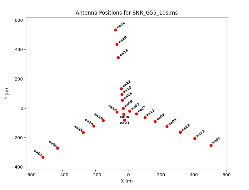
Antenna plot showing the configuration during the observing session.
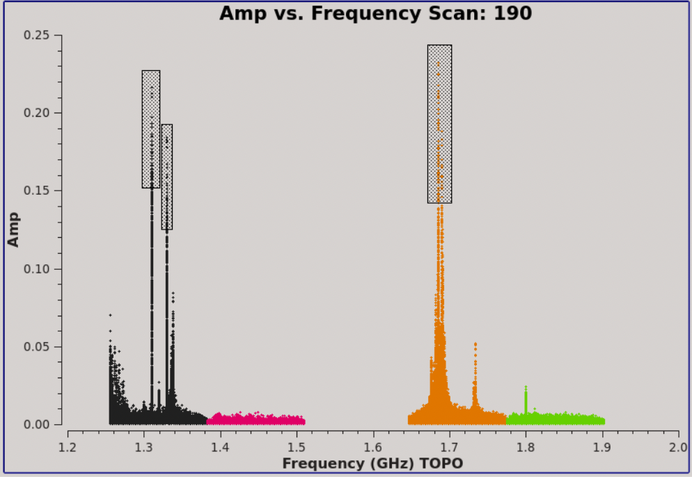
Plotms image of scan 190 showing strong RFI spikes in amplitude for several spectral windows.
Also note that 3C147 is used for both flux density and bandpass calibration.
It's important to be aware that the antennas have both a name and an ID associated with them. For example antenna ID 15 is named ea19 (the ea stemming from the Expanded VLA project). When specifying an antenna within a task parameter, we will primarily reference them by name.
We can see the antenna configuration for this observing session by using plotants:
# In CASA
plotants(vis='SNR_G55_10s.ms', figfile='SNR_G55_10s.plotants.png')
Figure 1 shows that antennas ea01, ea03, and ea18 were on the extreme ends of the west, east, and north arms, respectively. The antenna position diagram is particularly useful as a guide to help determine which antenna to use as the reference antenna later during calibration. Antennas on station 8 of each arm (N08, E08, W08) do not get moved during array re-configurations; they can, therefore, at times be good choices as reference antennas. In this case, we'll probably want to choose something closer to the center of the array with no shadowing.
We may also inspect the raw data using plotms. To start with, lets look at a subset of scans on the supernova remnant:
# In CASA
plotms(vis='SNR_G55_10s.ms', scan='30,75,120,165,190,235,303', antenna='ea24', xaxis='freq',
       yaxis='amp', coloraxis='spw', iteraxis='scan')
- coloraxis='spw': Parameter indicates that a different color will be assigned to each spectral window.
- antenna='ea24' : We chose only information for antenna ea24.
- iteraxis='scan': Parameter tells plotms to display a new plot for each scan.
Progressing through to scan 190 (by using the green triangle video button in the bottom of plotms), we can see there is significant time and frequency variable RFI present in the observing session. The RFI is discerned by the large spikes in amplitude and several spectral windows are badly affected. To determine which spectral windows, click on the Mark Regions tool at the bottom of the plotms GUI (the open box with a green plus sign) and use the mouse to select a few of the highest-amplitude points in each of the spectral windows (Figure 2). Click on the Locate button (magnifying glass on white background). Information about the selected areas should now display in the logger window. For example:
 INFO PlotMS Frequency in [1.30517 1.31368] or [1.32584 1.33313] or [1.68146 1.69544], Amp in [0.132051 0.223077] or [0.124359 0.188034] or [0.139316 0.237179]:
 INFO PlotMS Scan=190 Field=G55.7+3.4[1] Time=2010/08/23/05:19:58.0 BL=ea01@W09 & ea24@W05[0&19]  Spw=0 Chan=27 Freq=1.31 Corr=LR X=1.31 Y=0.139029   (110/144/110)
 INFO PlotMS Scan=190 Field=G55.7+3.4[1] Time=2010/08/23/05:19:58.0 BL=ea03@E09 & ea24@W05[2&19]  Spw=0 Chan=27 Freq=1.31 Corr=LL X=1.31 Y=0.145391   (623/144/623)
 INFO PlotMS Scan=190 Field=G55.7+3.4[1] Time=2010/08/23/05:19:58.0 BL=ea04@W01 & ea24@W05[3&19]  Spw=0 Chan=27 Freq=1.31 Corr=LL X=1.31 Y=0.166033   (879/144/879)
 INFO PlotMS Scan=190 Field=G55.7+3.4[1] Time=2010/08/23/05:19:58.0 BL=ea04@W01 & ea24@W05[3&19]  Spw=0 Chan=37 Freq=1.33 Corr=LR X=1.33 Y=0.131179   (918/144/918)
 INFO PlotMS Scan=190 Field=G55.7+3.4[1] Time=2010/08/23/05:19:58.0 BL=ea07@E05 & ea24@W05[5&19]  Spw=0 Chan=27 Freq=1.31 Corr=RL X=1.31 Y=0.14596    (1389/144/1389)
 INFO PlotMS Scan=190 Field=G55.7+3.4[1] Time=2010/08/23/05:19:58.0 BL=ea07@E05 & ea24@W05[5&19]  Spw=0 Chan=27 Freq=1.31 Corr=LL X=1.31 Y=0.142578   (1391/144/1391)
 INFO PlotMS Scan=190 Field=G55.7+3.4[1] Time=2010/08/23/05:19:58.0 BL=ea09@E06 & ea24@W05[7&19]  Spw=0 Chan=27 Freq=1.31 Corr=RR X=1.31 Y=0.141398   (1900/144/1900)
 INFO PlotMS Scan=190 Field=G55.7+3.4[1] Time=2010/08/23/05:19:58.0 BL=ea12@E08 & ea24@W05[10&19] Spw=0 Chan=37 Freq=1.33 Corr=LR X=1.33 Y=0.133163   (2710/144/2710)
 INFO PlotMS Scan=190 Field=G55.7+3.4[1] Time=2010/08/23/05:19:58.0 BL=ea13@N07 & ea24@W05[11&19] Spw=0 Chan=37 Freq=1.33 Corr=RR X=1.33 Y=0.129079   (2964/144/2964)
 INFO PlotMS Scan=190 Field=G55.7+3.4[1] Time=2010/08/23/05:19:58.0 BL=ea15@W06 & ea24@W05[12&19] Spw=0 Chan=27 Freq=1.31 Corr=RR X=1.31 Y=0.135901   (3180/144/3180)
 INFO PlotMS Scan=190 Field=G55.7+3.4[1] Time=2010/08/23/05:19:58.0 BL=ea16@W02 & ea24@W05[13&19] Spw=0 Chan=27 Freq=1.31 Corr=RR X=1.31 Y=0.17187    (3436/144/3436)
 INFO PlotMS Scan=190 Field=G55.7+3.4[1] Time=2010/08/23/05:19:58.0 BL=ea16@W02 & ea24@W05[13&19] Spw=0 Chan=27 Freq=1.31 Corr=LR X=1.31 Y=0.155113   (3438/144/3438)
 INFO PlotMS Scan=190 Field=G55.7+3.4[1] Time=2010/08/23/05:19:58.0 BL=ea16@W02 & ea24@W05[13&19] Spw=0 Chan=27 Freq=1.31 Corr=LL X=1.31 Y=0.142598   (3439/144/3439)
 INFO PlotMS Scan=190 Field=G55.7+3.4[1] Time=2010/08/23/05:19:58.0 BL=ea19@W04 & ea24@W05[15&19] Spw=0 Chan=27 Freq=1.31 Corr=LR X=1.31 Y=0.154241   (3950/144/3950)
 INFO PlotMS Scan=190 Field=G55.7+3.4[1] Time=2010/08/23/05:19:58.0 BL=ea19@W04 & ea24@W05[15&19] Spw=0 Chan=27 Freq=1.31 Corr=LL X=1.31 Y=0.178607   (3951/144/3951)
 INFO PlotMS Scan=190 Field=G55.7+3.4[1] Time=2010/08/23/05:19:58.0 BL=ea19@W04 & ea24@W05[15&19] Spw=0 Chan=37 Freq=1.33 Corr=RR X=1.33 Y=0.126879   (3988/144/3988)
 INFO PlotMS Scan=190 Field=G55.7+3.4[1] Time=2010/08/23/05:19:58.0 BL=ea21@E01 & ea24@W05[16&19] Spw=0 Chan=27 Freq=1.31 Corr=RL X=1.31 Y=0.144868   (4205/144/4205)
 INFO PlotMS Scan=190 Field=G55.7+3.4[1] Time=2010/08/23/05:19:58.0 BL=ea21@E01 & ea24@W05[16&19] Spw=0 Chan=27 Freq=1.31 Corr=LL X=1.31 Y=0.158044   (4207/144/4207)
 INFO PlotMS Scan=190 Field=G55.7+3.4[1] Time=2010/08/23/05:19:58.0 BL=ea22@N04 & ea24@W05[17&19] Spw=0 Chan=37 Freq=1.33 Corr=RR X=1.33 Y=0.18105    (4500/144/4500)
<snip>
 INFO PlotMS Scan=190 Field=G55.7+3.4[1] Time=2010/08/23/05:21:08.0 BL=ea22@N04 & ea24@W05[17&19] Spw=2 Chan=19 Freq=1.686 Corr=RR X=1.686 Y=0.195303 (10060/169/4428)
 INFO PlotMS Scan=190 Field=G55.7+3.4[1] Time=2010/08/23/05:21:08.0 BL=ea22@N04 & ea24@W05[17&19] Spw=2 Chan=19 Freq=1.686 Corr=RL X=1.686 Y=0.19185  (10061/169/4429)
 INFO PlotMS Scan=190 Field=G55.7+3.4[1] Time=2010/08/23/05:21:08.0 BL=ea22@N04 & ea24@W05[17&19] Spw=2 Chan=21 Freq=1.69 Corr=RR X=1.69 Y=0.169598   (10068/169/4436)
 INFO PlotMS Scan=190 Field=G55.7+3.4[1] Time=2010/08/23/05:21:17.5 BL=ea08@N01 & ea24@W05[6&19]  Spw=2 Chan=19 Freq=1.686 Corr=LR X=1.686 Y=0.157531 (7246/170/1614)
 INFO PlotMS Scan=190 Field=G55.7+3.4[1] Time=2010/08/23/05:21:17.5 BL=ea10@N03 & ea24@W05[8&19]  Spw=2 Chan=19 Freq=1.686 Corr=LL X=1.686 Y=0.15168  (7759/170/2127)
 INFO PlotMS Scan=190 Field=G55.7+3.4[1] Time=2010/08/23/05:21:17.5 BL=ea15@W06 & ea24@W05[12&19] Spw=2 Chan=19 Freq=1.686 Corr=LR X=1.686 Y=0.202071 (8782/170/3150)
 INFO PlotMS Scan=190 Field=G55.7+3.4[1] Time=2010/08/23/05:21:17.5 BL=ea18@N09 & ea24@W05[14&19] Spw=2 Chan=21 Freq=1.69 Corr=RR X=1.69 Y=0.159526   (9300/170/3668)
 INFO PlotMS Scan=190 Field=G55.7+3.4[1] Time=2010/08/23/05:21:17.5 BL=ea19@W04 & ea24@W05[15&19] Spw=2 Chan=19 Freq=1.686 Corr=RR X=1.686 Y=0.192973 (9548/170/3916)
 INFO PlotMS Scan=190 Field=G55.7+3.4[1] Time=2010/08/23/05:21:17.5 BL=ea19@W04 & ea24@W05[15&19] Spw=2 Chan=19 Freq=1.686 Corr=LR X=1.686 Y=0.155768 (9550/170/3918)
 INFO PlotMS Scan=190 Field=G55.7+3.4[1] Time=2010/08/23/05:21:17.5 BL=ea19@W04 & ea24@W05[15&19] Spw=2 Chan=19 Freq=1.686 Corr=LL X=1.686 Y=0.147995 (9551/170/3919)
 INFO PlotMS Scan=190 Field=G55.7+3.4[1] Time=2010/08/23/05:21:17.5 BL=ea22@N04 & ea24@W05[17&19] Spw=2 Chan=19 Freq=1.686 Corr=RR X=1.686 Y=0.199225 (10060/170/4428)
 INFO PlotMS Scan=190 Field=G55.7+3.4[1] Time=2010/08/23/05:21:17.5 BL=ea22@N04 & ea24@W05[17&19] Spw=2 Chan=19 Freq=1.686 Corr=RL X=1.686 Y=0.193489 (10061/170/4429)
 INFO PlotMS Scan=190 Field=G55.7+3.4[1] Time=2010/08/23/05:21:17.5 BL=ea22@N04 & ea24@W05[17&19] Spw=2 Chan=21 Freq=1.69 Corr=RR X=1.69 Y=0.179036   (10068/170/4436)
 INFO PlotMS Scan=190 Field=G55.7+3.4[1] Time=2010/08/23/05:21:17.5 BL=ea24@W05 & ea25@N02[19&20] Spw=2 Chan=19 Freq=1.686 Corr=RL X=1.686 Y=0.156535 (10573/170/4941)
 INFO PlotMS Scan=190 Field=G55.7+3.4[1] Time=2010/08/23/05:21:17.5 BL=ea24@W05 & ea25@N02[19&20] Spw=2 Chan=21 Freq=1.69 Corr=RR X=1.69 Y=0.140293   (10580/170/4948)
 INFO PlotMS Found 287 points (287 unflagged) among 202752 in 0.01s.
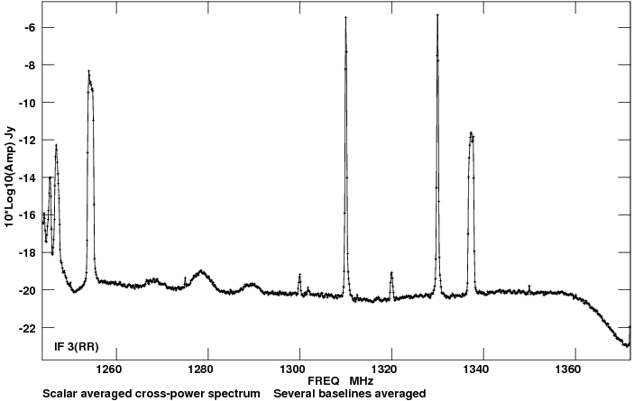
Amplitude vs. frequency plot of a portion of the L-band spectrum, showing RFI spikes from different sources.
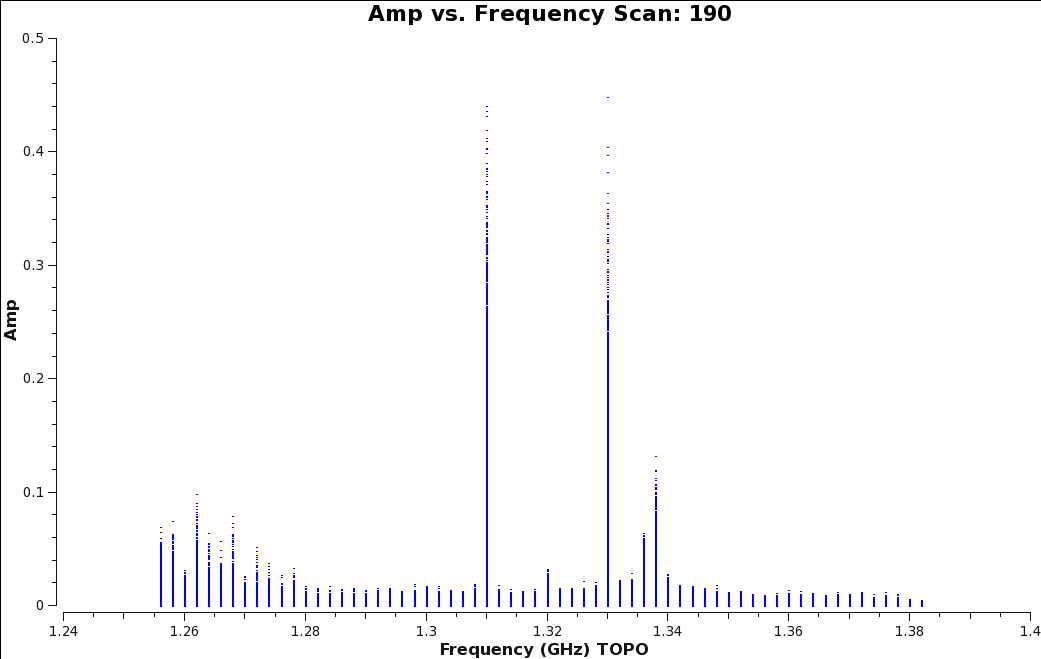
Amplitude vs. frequency plot of L-Band, spectral window 0, for scan 190. Generated by running the command "plotms(vis='SNR_G55_10s.ms', spw='0', scan='190', xaxis='freq', yaxis='amp')" within CASA.
Reviewing the log output, we can see that spw 0 and 2 are affected the worst by RFI. We also get the corresponding frequency where the RFI is present, which appears to be 1.31 and 1.33 GHz for spectral window 0, and 1.686 GHz for spectral window 2. This information is important, especially when flagging data interactively as we will be doing towards the end of this guide.
The VLA has obtained RFI sweeps over its full frequency range. The results are available on the Radio Frequency Interference website. Most of the RFI features can be identified as radar, communications, satellites, airplanes, or birdies (i.e., RFI generated by the VLA electronics itself). For our observations, we inspect the L-band specific RFI plots website and find that the 1310 and 1330 MHz features are due to FAA ASR radars, while the one at 1686 MHz is most likely due to a GOES weather satellite. We can compare the plots of the FAA ASR radar from the website (Figure 3a), with that of spw 0 (Figure 3b), and see that the spikes are practically identical and fall within the same frequencies.
Identifying Problematic Antennas from the Operator Logs
We first check the operator log for the observing session to see if there were any issues noted during the run that need to be addressed. The logs are available from the VLA operator log website. Here is the link for the observing log file for our observing session.
The log has various pieces of information including the start/end times for the observing session, frequency bands used, weather, baseline information for recently moved antennas, and any outages or issues that may have been encountered. We see that antenna ea07 may need position corrections (see one of our calibration tutorials, IRC+10216, on how to fix this), and several antennas (ea06, ea17, ea20, and ea26) are missing an L-Band receiver. Antenna 07 position corrections will need to be applied during data calibration and will not be covered in this tutorial. Additionally, the antennas with missing receivers were already removed from the dataset used here (as explained in the above section Obtaining the Data), so we can continue with online flagging.
Online Flags
At the time of importing from the SDM-BDF raw data to a MS, we chose to process the online flags from the Flags.xml file to the FLAG_CMD sub-table within the MS. We also created the SNR_G55.ms.onlineflags.txt file, a plain text document that includes the list of online flags.
The Flags.xml file holds information of flags created during the observing session, such as subreflector issues and antennas not being on source. We will now apply these online flags to the data by employing flagcmd, but first, let's create a plot of the flags to get an idea of what will be flagged.
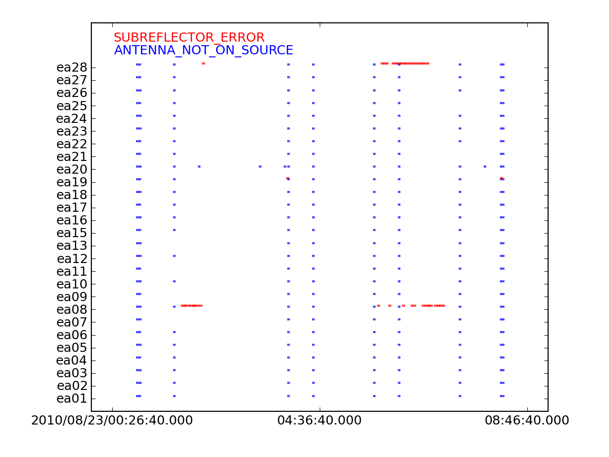
Online Flags
# In CASA
flagcmd(vis='SNR_G55_10s.ms', inpmode='table', reason='any', action='plot', plotfile='flaggingreason_vs_time.png')
Open the flaggingreason_vs_time.png with your favorite image viewing program. Figure 4 shows several instances of online flagging. Most notably, ea28 and ea08 had some subreflector issues throughout the observing session. Online flags are instances of possible missing data, including:
- ANTENNA_NOT_ON_SOURCE
The VLA antennas have slewing speeds of 40 degrees per minute in azimuth and 20 degrees per minute in elevation. Some antennas are slower than others and may take a few more seconds to reach the next source. The antennas can also take a few seconds to settle down due to small oscillations after having slewed.
- SUBREFLECTOR_ERROR
The Focus Rotation Mount (FRM), located at the apex of the antenna, is responsible for focusing the incoming radio signal to the corresponding receiver. They can at times have issues with their focus and/or rotation axes.
Now that we've plotted the online flags, we will apply them to the MS.
# In CASA
flagcmd(vis='SNR_G55_10s.ms', inpmode='table', reason='any', action='apply', flagbackup=False)
- inpmode='table': Will use the online-flags imported to the FLAG_CMD sub-table from the Flags.xml file. This was done during the importing of our data with importasdm. Note that the FLAG_CMD sub-table already includes a 1.5 second time buffer, as was requested during the importing of the data (parameter tbuff=1.5).
The CASA logger should report the progress as the task applies these flags in segments. Once finished, it will report the percentage of flagged data. The terminal window will display warnings about the four missing antennas; this is expected, as we had previously removed the antennas during the split task.
Alternatively, we could have applied the online flags from the text file (SNR_G55.ms.onlineflags.txt) created during the importing of the data. The one caveat when it comes to applying flags from a list is not being able to un-apply them (setting parameter action='unapply' within flagcmd). Transferring the flags to the FLAGS_CMD table before applying them does allow for the use of the un-apply feature. For convenience, we provide the command for applying online flags from a list (don't run the following command in CASA):
flagcmd(vis='SNR_G55_10s.ms', inpmode='list', inpfile='SNR_G55.ms.onlineflags.txt', reason='any', action='apply', flagbackup=False)
Shadowed Antennas
The VLA D-configuration is the most compact; there may be, therefore, instances where one antenna blocks, or shadows, another. For more on shadowing, please refer to the antenna shadowing section in the Guide to Observing with the VLA. Generally, observing sources at 40 degrees elevation and higher will result in less shadowing. We will create a plot of elevation vs. time by using the plotms task and note the elevation of the radio sources we observed.
# In CASA
plotms(vis='SNR_G55_10s.ms', xaxis='time', yaxis='elevation', antenna='0&1;2&3', spw='*:31',
       coloraxis='field', title='Elevation vs. Time', plotfile='Elevation_vs_Time.png')
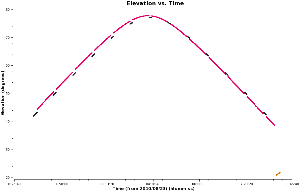
Elevation vs Time
Figure 5 shows that most of the sources were at or above 40 degrees in elevation; accordingly, we expect a minimal amount of shadowing. The flux density / bandpass calibrator 3C147 was observed towards the end of the session, which could result in some shadowing of antennas due to its low elevation of about 20–22 degrees.
Task flagdata (CASA Cookbook 3.4) can determine and flag shadowed antennas by their location and observing direction:
# In CASA
flagdata(vis='SNR_G55_10s.ms', mode='shadow', tolerance=0.0, flagbackup=False)
- mode='shadow': has a subparameter tolerance=0.0 that controls how many meters of shadowing overlap is allowed
The logger will report on the percentage of flagged data due to shadowing. In this observing session, as expected, there does not appear to be much data affected by shadowing.
Zero-Amplitude Data
In addition to shadowing, there may be times during which the correlator writes out pure zero-valued data. In order to remove this bad data, we run flagdata to remove any pure zeroes:
# In CASA
flagdata(vis='SNR_G55_10s.ms', mode='clip', clipzeros=True, flagbackup=False)
- mode='clip': is used to flag all values below a given threshold. With clipzeros=True this mode will flag exact zero values that are sometimes being produced by the VLA correlator.
Inspecting the logger output generated by flagdata shows that there is a small quantity of zero-valued data present in this MS.
Quacking
Now we utilize the flagdata task one more time to run quacking mode.
It's common for the array to settle down at the start of a scan. Quacking is used to remove data at scan boundaries, the same edit can be applied to all scans for all baselines.
# In CASA
flagdata(vis='SNR_G55_10s.ms', mode='quack', quackinterval=5.0, quackmode='beg', flagbackup=False)
- quackmode='beg' : Data from the start of each scan will be flagged.
- quackinterval=5.0: Flag the first 5 seconds of every scan.
Backup Data - Flagmanager
Flags can be backed up in a file MS.flagversions that is related to the MS. For our MS, the related flag backups are stored in SNR_G55_10s.ms.flagversions.
Note: flags that are applied to the data are contained in the MS. MS.flagversions only contains backup flags that can be restored if required.
Most flagging tasks, like flagdata, offer a flagbackup parameter that controls whether or not the current flags are being backed up in MS.flagversions before new (additional) flags will be applied. Backup flags can also be manually saved to, or restored from, MS.flagversions using the flagmanager task.
Now that we've applied online flags, clipped zero amplitude data, removed shadowed data, and quacked the data, we will create a backup of the flags, setting the parameter versionname='after_online_flagging' :
# In CASA
flagmanager(vis='SNR_G55_10s.ms', mode='save', versionname='after_online_flagging')
From here onward, if we make a mistake, we can always revert back to this flag version of the MS by setting parameter mode='restore' and providing the version name we want to revert back to, such as:
flagmanager(vis='SNR_G55_10s.ms', mode='restore', versionname='after_online_flagging')
Hanning-Smoothing
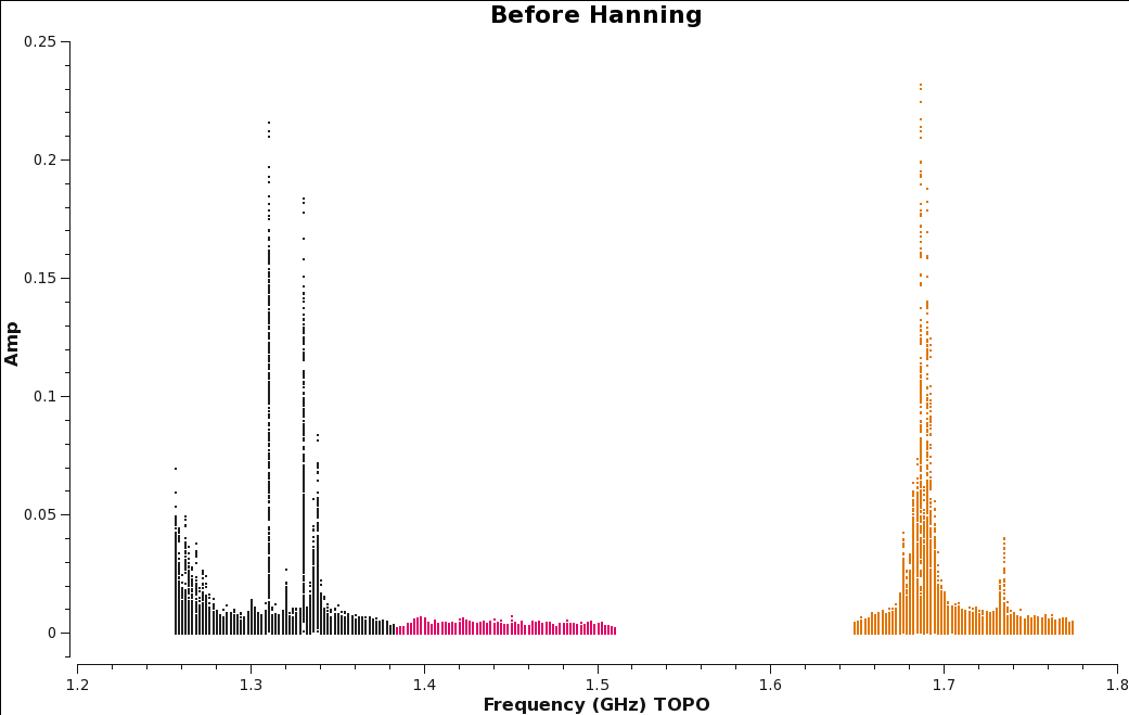
Plot of amplitude vs. frequency before Hanning smoothing data.
Strong RFI sources can give rise to the Gibbs phenomenon. This is seen by ringing, a zig-zag pattern across the channels that neighbor the strong, usually narrow, RFI. To remedy this ringing across the frequency channels, we employ the hanningsmooth algorithm via the hanningsmooth2 task (an implementation based on mstransform). Hanning-smoothing applies a triangle kernel across the pattern which diminishes the ringing, reducing the number of channels that may look bad and get flagged. This smoothing procedure will also decrease the spectral resolution by a factor of two.
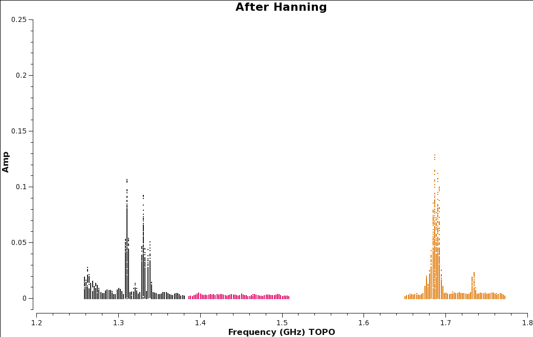
Plot of amplitude vs. frequency after Hanning smoothing data.
The task requires the creation of a new MS. We will be creating a new MS called SNR_G55_10s-hanning.ms. As Hanning-smoothing will remove amplitude spikes it is, therefore, not recommended for spectral analysis related science such as strong narrow maser lines.
Let's create before (Figure 6a) and after images (Figure 6b) with the plotms task to see the effect.
# In CASA
plotms(vis='SNR_G55_10s.ms', scan='190', antenna='ea24', spw='0~2',
       xaxis='freq', yaxis='amp', coloraxis='spw', title='Before Hanning',
       correlation='RR,LL', plotrange=[1.2,1.8,-0.01,0.25],
       plotfile='amp_v_freq.beforeHanning.png')
# In CASA
hanningsmooth2(vis='SNR_G55_10s.ms', outputvis='SNR_G55_10s-hanning.ms', datacolumn='data')
# In CASA
plotms(vis='SNR_G55_10s-hanning.ms', scan='190', antenna='ea24', spw='0~2',
       xaxis='freq', yaxis='amp', coloraxis='spw', title='After Hanning',
       correlation='RR,LL', plotrange=[1.2,1.8,-0.01,0.25],
       plotfile='amp_v_freq.afterHanning.png')
Figure 6b shows the effect of applying Hanning-smoothing. Notice that single channel RFI has spread into three channels. This spreading of RFI to other channels will ultimately result in a little more data being flagged.
Automatic RFI excision
Now that we're done with online flagging, we can move on to removing some of the RFI present with auto-flagging algorithms used within flagdata, TFCrop and rflag. For further details on the two algorithm based tasks we will employ, please see the RFI presentation given at the 5th VLA Data Reduction Workshop.
TFCrop
Task flagdata's TFCrop is an algorithm that detects outliers in the 2D time-frequency plane and can operate on un-calibrated (non-bandpass corrected) data. TFCrop will iterate through segments of time and undergo several steps in order to find and excise different types of RFI (CASA Cookbook 3.4.2.7):
Step 1: Detect short-duration RFI spikes (narrow- and broad-band).
Step 2: Search for time-persistent RFI.
Step 3: Search for time-persistent, narrow-band RFI.
Step 4: Search for low-level wings of very strong RFI.
We will apply the auto-flagging TRCrop algorithm for each spectral window. With TFCrop, it's a good idea to first inspect a small portion of data and review what and how much will be flagged. Once you are comfortable with the results, you can apply the algorithm to the remaining data. We will walk through the first spw and then include the remaining spws with the same command. First plot the corrected data for scan 190 (Figure 7) with all spectral windows so we can compare the data before and after TFCrop.
# In CASA
plotms(vis='SNR_G55_10s-hanning.ms', scan='190', antenna='ea24', xaxis='freq', iteraxis='scan', yaxis='amp',
       ydatacolumn='data', plotfile='amp_v_freq_before_tfcrop.png', title='Before TFCrop',
       coloraxis='spw', plotrange=[1.2,2,-0.01,0.25])
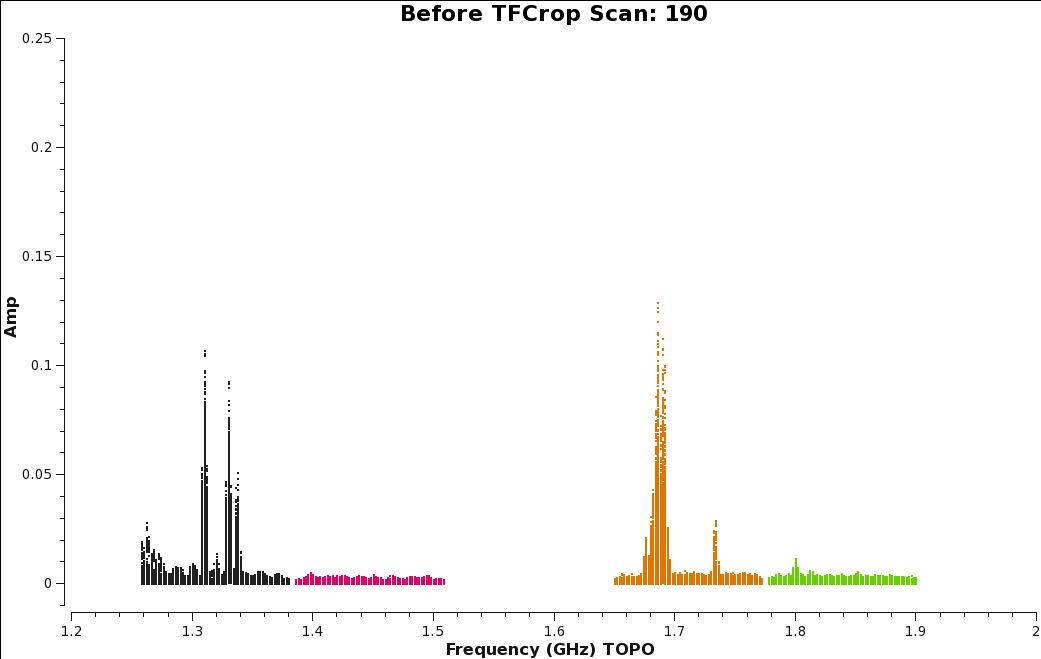
Amplitude vs. Frequency plot of Scan 190, before the TFCrop algorithm is applied.
The following are a set of flagdata commands which have been found to work reasonably well with these data. Please take some time to play with the parameters and the plotting capabilities. Since these runs set parameters display='both' and action='calculate', the flags are displayed but not actually written to the MS. This allows one to try different sets of parameters before actually applying the flags to the data.
Some representative TFCrop plots are also displayed (Figure 8). Each column displays an individual polarization product; all four polarizations are, from left to right, RR, RL, LR, and LL. The first row shows the data with current flags applied and the second includes the flags generated by flagdata. The x-axis is channel number (the spectral window ID is displayed in the top title) and the y-axis of the first two rows is all integrations included in a time segment, set by the parameter ntime. These are the data considered by the TFCrop algorithm during its flagging process, and changes in ntime will have some (relatively small) effect on what data are flagged.
Each plot page displays data for a single baseline and time segment. The buttons at the bottom allow one to step through baseline (backward and forward), spw, scan, and field. Stop Display will continue the flagging operation without the GUI, and Quit aborts the run.
spw 0
# In CASA
flagdata(vis='SNR_G55_10s-hanning.ms', mode='tfcrop', spw='0',
         datacolumn='data', action='calculate',
         display='both', flagbackup=False)
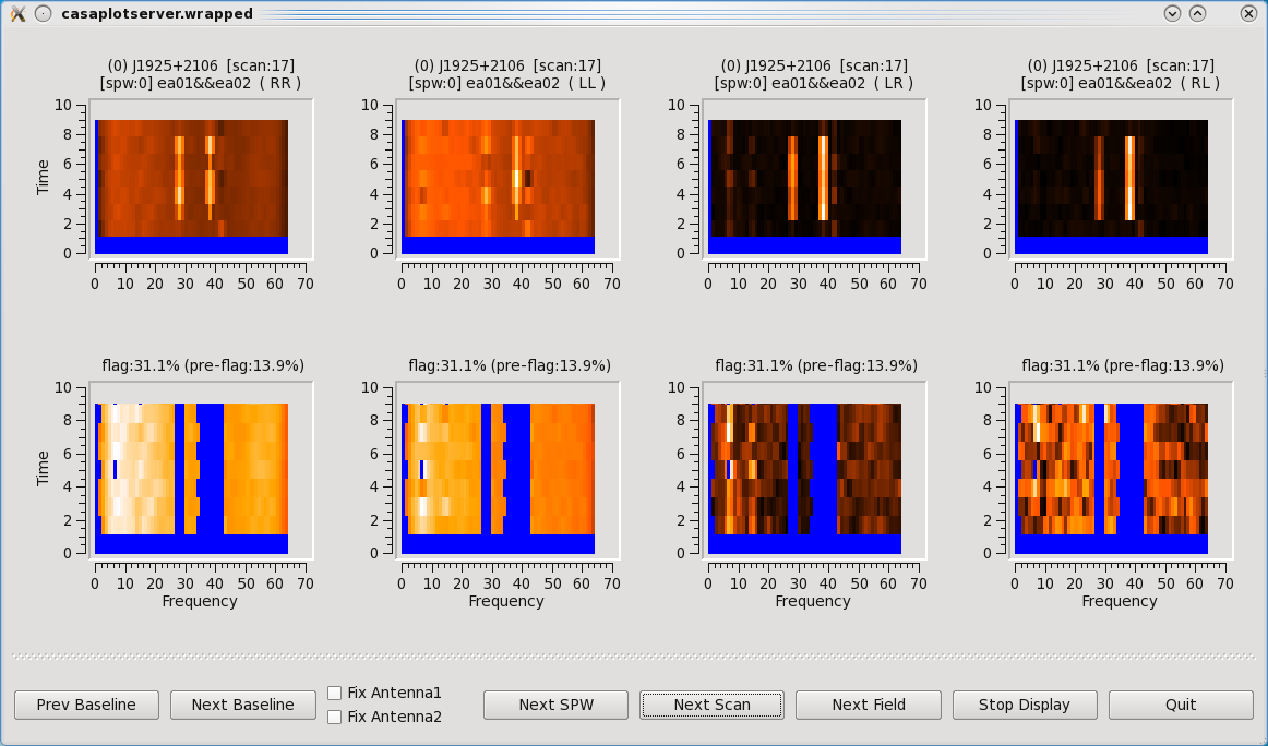
TFCrop flagging results. Top row before, bottom row, after TFCrop.
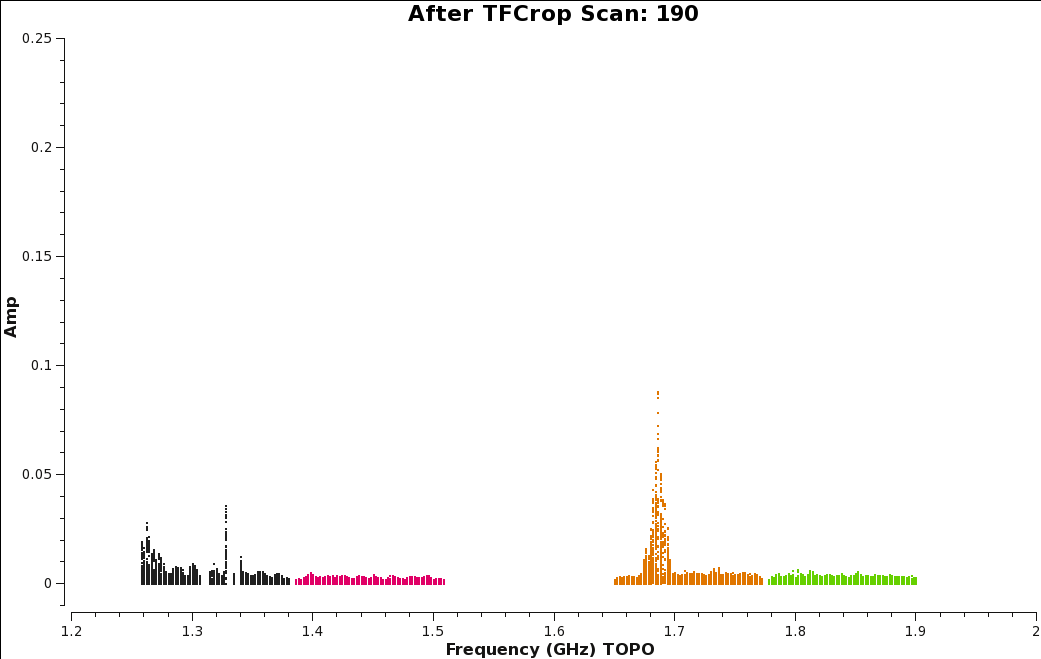
Plot of amplitude vs frequency showing the effects of applying TFCrop to our data, for scan 190.
Click on Next Scan until you reach scan 17. The bottom row illustrates the flagging that can be applied, represented by the additional blue areas. Iterate through several scans and baselines, and once you're done, click on the Quit button on the bottom right corner. Let's now apply these flags by changing the action parameter.
# In CASA
flagdata(vis='SNR_G55_10s-hanning.ms', mode='tfcrop', spw='0',
         datacolumn='data', action='apply',
         display='', flagbackup=False)
The logger will report the percentage of flagged data in the table selection. We can now apply the TFCrop algorithm to the remaining spectral windows.
spw 1, 2, 3
# In CASA
flagdata(vis='SNR_G55_10s-hanning.ms', mode='tfcrop', spw='1~3',
         datacolumn='data', action='apply',
         display='both', flagbackup=False)
Iterate through several scans and baselines, and once you're ready to apply the flags, click on Stop Display. After TFCrop has gone through and flagged some of the worst RFI, we can inspect the log report and take note of how much has been flagged.
We can also use plotms to review the effects of using TFCrop. Compare the plots before applying TFCrop (Figure 7) to the plot after applying TFCrop (Figure 9). Figure 9 shows great improvements, especially for spectral window 0 and 2, which had some of the worst RFI.
# In CASA
plotms(vis='SNR_G55_10s-hanning.ms', scan='190', antenna='ea24', xaxis='freq', iteraxis='scan', yaxis='amp',
       ydatacolumn='data', plotfile='amp_v_freq_after_tfcrop.png', title='After TFCrop',
       correlation='RR,LL', coloraxis='spw', plotrange=[1.2,2,-0.01,0.25])
Flagging Summary
We now calculate the amount of flagged data so far in our Measurement Set by using the flagdata task with parameter mode='summary' and assign the returned Python dictionary to the variable flagInfo. We then parse the dictionary to print some of the flagging statistics.
# In CASA
flagInfo = flagdata(vis='SNR_G55_10s-hanning.ms', mode='summary')
# In CASA
print("\n %2.1f%% of G55.7+3.4, %2.1f%% of 3C147, and %2.1f%% of J1925+2106 are flagged. \n" %
     (100.0 * flagInfo['field']['G55.7+3.4']['flagged'] / flagInfo['field']['G55.7+3.4']['total'],
     100.0 * flagInfo['field']['0542+498=3C147']['flagged'] / flagInfo['field']['0542+498=3C147']['total'],
     100.0 * flagInfo['field']['J1925+2106']['flagged'] / flagInfo['field']['J1925+2106']['total']))
# In CASA
print("Spectral windows are flagged as follows:")

for spw in range(0,4):
     print("SPW %s: %2.1f%%" % (spw, 100.0 * flagInfo['spw'][str(spw)]['flagged'] / flagInfo['spw'][str(spw)]['total']))
We can now move to the other auto-flagging algorithm, rflag.
RFlag
RFlag, like TFCrop, is an autoflag algorithm which uses a sliding window statistical filter. Data is iterated through in segments of time where statistics are accumulated and thresholds calculated.
WARNING: It is important to not assume that rflag can run on your target. This is especially important for spectral lines, as it may mistake them for interference.
Task flagdata (rflag) should be executed on calibrated data only. For more details, please see Emmanuel Momjian's presentation on VLA Data Reduction Techniques and Calibration given during the 5th VLA Data Reduction Workshop.
In order to get the best possible result from the automatic RFI excision with flagdata's mode rflag, we will first apply bandpass calibration to the MS. Since the RFI is time-variable, using the phase calibration source to make an average bandpass over the entire observing session will mitigate the amount of RFI present in the calculated bandpass. For the final calibration, we will use the designated bandpass source 3C147, which will give a much higher signal to noise in the bandpass. Since 3C147 was only observed in the last set of scans, it doesn't sample the time variability and would not provide a good average bandpass.
Since there are likely to be gain variations over the course of the observing session, we will run gaincal to solve for an initial set of antenna-based phases over a narrow range of channels. Those solutions will be applied to the data when the bandpass solutions are determined. While amplitude variations will have little effect on the bandpass solutions, it is important to solve for these phase variations with sufficient time resolution to prevent decorrelation when vector averaging the data in computing the bandpass solutions.
In order to choose a narrow range of channels for each spectral window, that are relatively RFI-free over the course of the observing session, we can look at the data with plotms. Note that it's important to solve only for phase using a narrow channel range, since an antenna-specific delay will cause the phase to vary with respect to frequency over the spectral window, perhaps by a substantial amount.
# In CASA
plotms(vis='SNR_G55_10s-hanning.ms', scan='42,65,88,11,134,157', antenna='ea24',
       xaxis='channel', yaxis='amp', iteraxis='spw')
Iterating over each spectral window plot, we will search for channel ranges with stable amplitudes. An example of a few appropriate channel ranges include:
SPW 0: 20-24
SPW 1: 49-52
SPW 2: 38-41
SPW 3: 41-44
Using these ranges, we run gaincal to calculate phase-only solutions that will be used as input during our initial bandpass calibration. Remember—the calibration tables we are creating now are so that we can use an automatic RFI flagging algorithm. Our final calibration tables will be generated later, after automated flagging. Here are the inputs for our initial pre-bandpass phase calibration:
# In CASA
gaincal(vis='SNR_G55_10s-hanning.ms', caltable='SNR_G55_10s-hanning.initPh', field='J1925+2106', solint=' int ',
        spw='0:20~24,1:49~52,2:38~41,3:41~44', refant='ea24', minblperant=3,
        minsnr=3.0, calmode='p')
- caltable='SNR_G55_10s-hanning.initPh': this is the output calibration table that will be written.
- field='J1925+2106': this is the phase calibrator we will use to calibrate the phases.
- solint=' int ': we request a solution for each 10-second integration.
- spw='0:20~24,1:49~52,2:38~41,3:41~44': note the syntax of this selection: a : is used to separate the SPW from channel selection and ~ is used to indicate an inclusive range.
- refant='ea24': we have chosen ea24 as the reference antenna after inspecting the antenna position diagram (see above). It is relatively close to the center of the array. Since the antennas in the very center have a high probability of being shadowed by nearby antennas, choose one that is not directly in the center. This is most important for the more compact (D, C) array configurations.
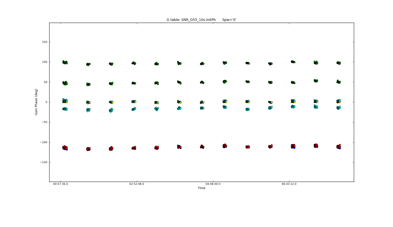
Gain Phase vs. Time for spw0, for four antennas.
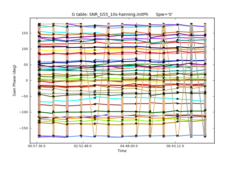
Gain Phase vs. Time for spw0, for all antennas, with plotsymbol='-', in order to connect the data points and inspect for phase jumps.
- minblperant=3: the minimum number of baselines which must be present to attempt a phase solution.
- minsnr=3.0: the minimum signal-to-noise a solution must have to be considered acceptable. Note that solutions which fail this test will cause these data to be flagged downstream of this calibration step.
- calmode='p': perform phase-only solutions.
Note that a number of solutions do not pass the requirements of the minimum 3 baselines (generating the terminal message "Insufficient unflagged antennas to proceed with this solve.") or minimum signal-to-noise ratio (outputting "n of x solutions rejected due to SNR being less than 3 ..."). The logger output indicates 320-324 solutions succeeded out of 387 attempted.
It's always a good idea to inspect the resulting calibration table with plotcal.
# In CASA
plotcal(caltable='SNR_G55_10s-hanning.initPh', xaxis='time', yaxis='phase', iteration='spw',
        antenna='ea01,ea05,ea10,ea24', plotrange=[-1,-1,-180,180])
Figure 10a shows the phases do not change much over the course of the observing session. In our last call to plotcal, we deliberately chose to only plot four antennas, as plotting all of them together will make the plot look convoluted, and this makes it difficult to determine any phase jumps that may be present. To remedy this, we will employ plotcal again with the plotsymbol parameter set to connect the data points.
# In CASA
plotcal(caltable='SNR_G55_10s-hanning.initPh', xaxis='time', yaxis='phase', iteration='spw',
        antenna='', plotsymbol = '-', plotrange=[-1,-1,-180,180])
Figure 10b may look to have phase jumps, but the V-shapes present are the program attempting to wrap the data points. As a user exercise, plot the phase from -180 to 0, and 0 to +180 to get the stable lines.
Now that we've determined our plots look fairly reasonable, we will create a time-averaged bandpass solution for the phase calibration source using the bandpass task.
# In CASA
bandpass(vis='SNR_G55_10s-hanning.ms', caltable='SNR_G55_10s-hanning.initBP', field='J1925+2106', solint=' inf ', combine='scan',
         refant='ea24', minblperant=3, minsnr=10.0, gaintable='SNR_G55_10s-hanning.initPh',
         interp='nearest', solnorm=False)
- solint=' inf ', combine='scan': the solution interval of infinite, up to the boundaries controlled by the combine parameter; this requests that the solution intervals be combined over scans, so that we will get one solution per antenna.
- gaintable= 'SNR_G55_10s-hanning.initPh': we will pre-apply the initial phase solutions.
- interp='nearest': by default, bandpass will use linear interpolation for pre-applied calibration. However, we want the nearest phase solution to be used for a given time.
Again, we can see that a number of solutions have been rejected by our choice of minsnr.
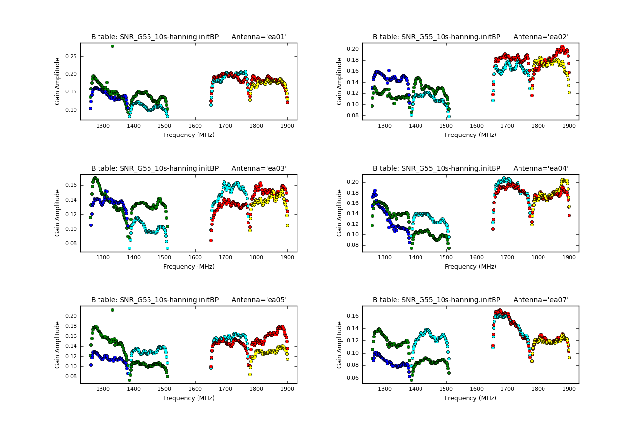
Bandpasses for antennas ea01 - ea07 (ea06 flagged)
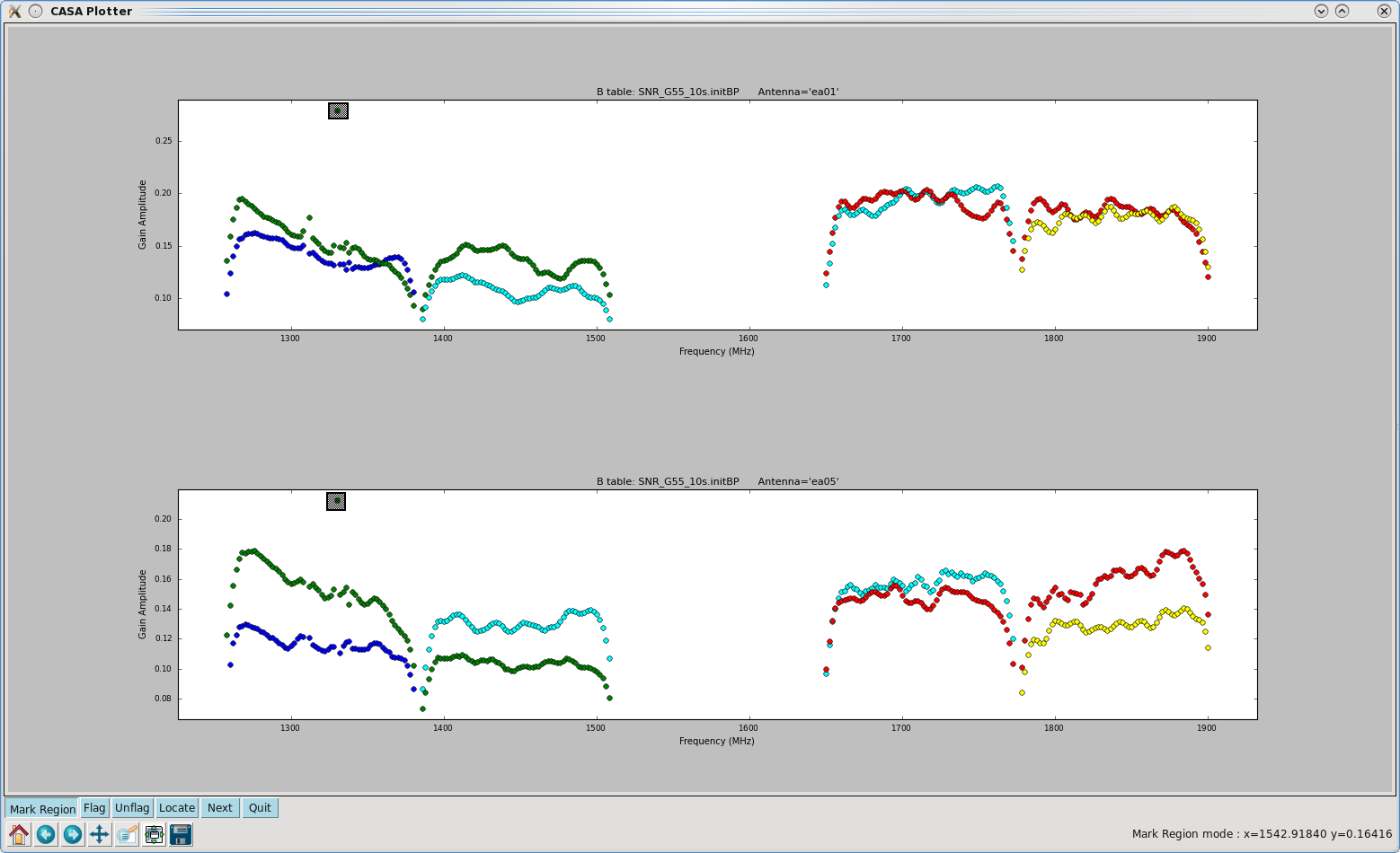
Interactive plotcal flagging of the offset points for ea01 and ea05.
Let us now inspect the resulting bandpass plots with plotcal.
# In CASA
plotcal(caltable='SNR_G55_10s-hanning.initBP', xaxis='freq', yaxis='amp',
        iteration='antenna', subplot=321)
- subplot=331: displays 3x3 plots per screen
We notice that antenna's ea01 and ea05 have a point that is offset from the rest (Figure 11). Let's plot just these two antennas, locate the point on the plot, and flag it interactively through plotcal. Please note that interactive flagging within plotcal will not create a backup, therefore it may be wise to use flagmanager before doing so.
# In CASA
plotcal(caltable='SNR_G55_10s-hanning.initBP', antenna='ea01,ea05', xaxis='freq',
        yaxis='amp', iteration='antenna', subplot=211)
We will highlight the points by clicking on the Mark Region button, drawing boxes over the points, and clicking on the Flag button. Before doing this, one could also get information on the points by clicking on the Locate button, which will display details about the highlighted regions (Figure 12). After having flagged the offset points, your plots should update.
We will now apply the bandpass calibration table using applycal.
# In CASA
applycal(vis='SNR_G55_10s-hanning.ms', gaintable='SNR_G55_10s-hanning.initBP', calwt=False)
This operation will flag data that correspond to flagged solutions, so applycal makes a backup version of the flags prior to operating on the data. Running applycal might take a little while.
Now that we have bandpass-corrected data, we will run flagdata in rflag mode (CASA Cookbook 3.4.2.8).
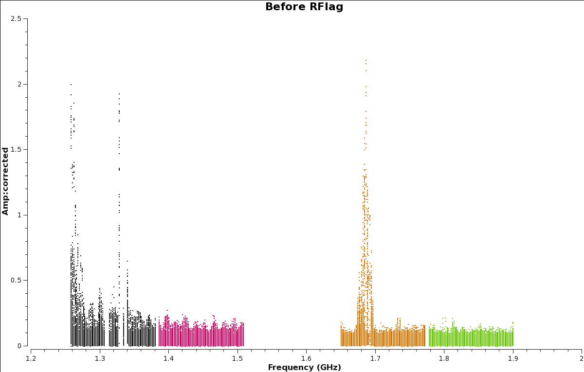
Amplitude vs. Frequency plot of scan 190, before RFlag is applied.
We will use flagdata with parameters mode='rflag', and action='calculate' to first review the amount of data to be flagged. We will also change the parameter datacolumn='corrected' since we've applied the bandpass corrections to the MS and, in the process, created the corrected_data column in the MS table.
spw 0
First, let's create a plot of our corrected data before we apply RFlag (Figure 13).
# In CASA
plotms(vis='SNR_G55_10s-hanning.ms', scan='190' , antenna='ea24',
xaxis='freq', yaxis='amp', ydatacolumn='corrected', coloraxis='spw',
title='Before RFlag', plotfile='amp_v_freq.beforeRFlag.png')
# In CASA
flagdata(vis='SNR_G55_10s-hanning.ms', mode='rflag', spw='0', datacolumn='corrected',
         action='calculate', display='both', flagbackup=False)
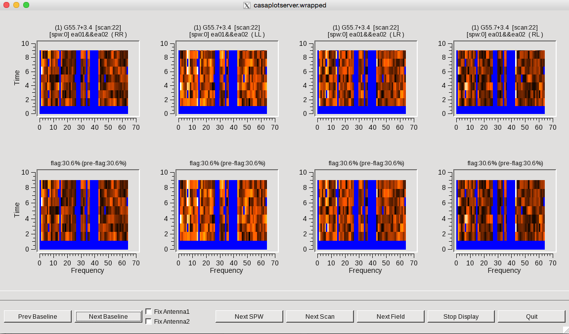
RFlag with Default Parameters for scan 22 (use the next scan, next baseline, and next field buttons to see this specific screen).
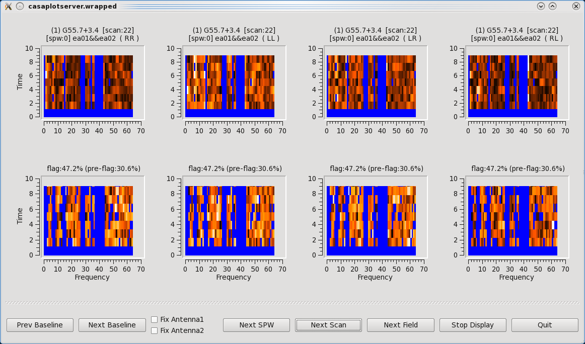
RFlag with freqdevscale=2.5, and timedevscale=3.5 for scan 22. We can see more data is being flagged with these more stringent values(use the next scan, next baseline, and next field buttons to see this specific screen).
After reviewing the calculated flags, we can see that a lot of RFI is being missed (Figure 14). We will need to modify the default parameters for this spectral window. Click on Quit on the lower right hand side of the window. Let's review the parameters for flagdata and modify them:
# In CASA, get the last called parameter values for flagdata
tget flagdata
# In CASA, inspect the inputs
inp
The default timedevscale and freqdevscale parameters of 5.0 are not flagging enough bad data. We can provide more stringent values to the time/freq deviation scales parameters. A value smaller than the default (5.0) will flag more data in either the time or frequency axis, as can be seen on the plots in the displayed window. A value larger than the default will result in less flagged data.
Since we know spw 0 has lots of RFI, we will change parameters freqdevscale=2.5 and timedevscale=3.5. We will also change parameter action='apply'. Note that we can always decide that this still isn't good enough and click on Quit to change our parameter values. Once the window opens, scroll to scan 22 (Figure 15), review what will be flagged, and click on Stop Display (as we did during TFCrop) to allow the task to continue with the flagging.
# In CASA
flagdata(vis='SNR_G55_10s-hanning.ms', mode='rflag', spw='0', datacolumn='corrected',
         freqdevscale=2.5, timedevscale=3.5, action='apply', display='both', flagbackup=False)
Although RFlag has done a pretty good job of finding the bad data, some still remains. One way to excise the remaining bad data is to use parameter mode='extend' feature in flagdata, which can extend flags along a chosen axis and removes islands of small data patches in the midst of flagged data. We first extend the flags across polarization so if any one polarization is flagged, all data for that time / channel will be flagged:
# In CASA
flagdata(vis='SNR_G55_10s-hanning.ms', mode='extend', spw='0', extendpols=True,
         action='apply', display='', flagbackup=False)
Now we extend the flags in time and frequency,using the parameters growtime and growfreq. For this data, the rflag algorithm seems most likely to miss RFI that should be flagged along more of the time axis. We will try with parameter growtime=50.0, which will flag all data for a given channel if more than 50% of that channel's time is already flagged, and parameter growfreq=90.0, which will flag the entire spectrum for an integration if more than 90% of the channels in that integration are already flagged.
# In CASA
flagdata(vis='SNR_G55_10s-hanning.ms', mode='extend', spw='0', growtime=50.0,
         growfreq=90.0, action='apply', display='', flagbackup=False)
spw 1, 2, and 3
Now, let's work on SPW's 1,2, and 3. We've chosen parameter display='both' in order to first review the flags to decide if too much or too little is being flagged. We can always click on Quit and decide to change parameters freqdevscale and timedevscale as we did with spectral window 0. Note that spw 2 has these parameters set lower than spw 1 and 3, as it contains more RFI. To allow the flagging to continue, click on Stop Display.
# In CASA
flagdata(vis='SNR_G55_10s-hanning.ms', mode='rflag',  spw='1,3', datacolumn='corrected',
         freqdevscale=4.0, timedevscale=4.0, action='apply', display='both', flagbackup=False)
# In CASA
flagdata(vis='SNR_G55_10s-hanning.ms', mode='extend', spw='1,3', extendpols=True,
         action='apply', display='', flagbackup=False)
# In CASA
flagdata(vis='SNR_G55_10s-hanning.ms', mode='extend', spw='1,3', growtime=50.0,
         growfreq=90.0, action='apply', display='', flagbackup=False)
# In CASA
flagdata(vis='SNR_G55_10s-hanning.ms', mode='rflag',  spw='2', datacolumn='corrected',
         freqdevscale=2.5, timedevscale=2.5, action='apply', display='both', flagbackup=False)

Plot of amplitude vs. frequency of scan 190, after having run RFlag.
# In CASA
flagdata(vis='SNR_G55_10s-hanning.ms', mode='extend', spw='2', extendpols=True,
         action='apply', display='', flagbackup=False)
# In CASA
flagdata(vis='SNR_G55_10s-hanning.ms', mode='extend', spw='2', growtime=50.0,
         growfreq=90.0, action='apply', display='', flagbackup=False)
Let's create an after RFlag plot to see the improvements (Figure 16). Compare the resulting plot to the before TFCrop plot (Figure 13).
# In CASA
plotms(vis='SNR_G55_10s-hanning.ms', scan='190' , antenna='ea24',
xaxis='freq', yaxis='amp', ydatacolumn='corrected', coloraxis='spw', title='After RFlag',
plotfile='amp_v_freq.afterRFlag.png', plotrange=[1.2,2,0,2.5])
We will now plot amplitude vs. baseline, and look for outliers which we may be able to flag.
# In CASA
plotms(vis='SNR_G55_10s-hanning.ms', scan='30,75,120,165,190,235,303', xaxis='baseline', yaxis='amp',
ydatacolumn='corrected', iteraxis='scan', coloraxis = 'baseline')
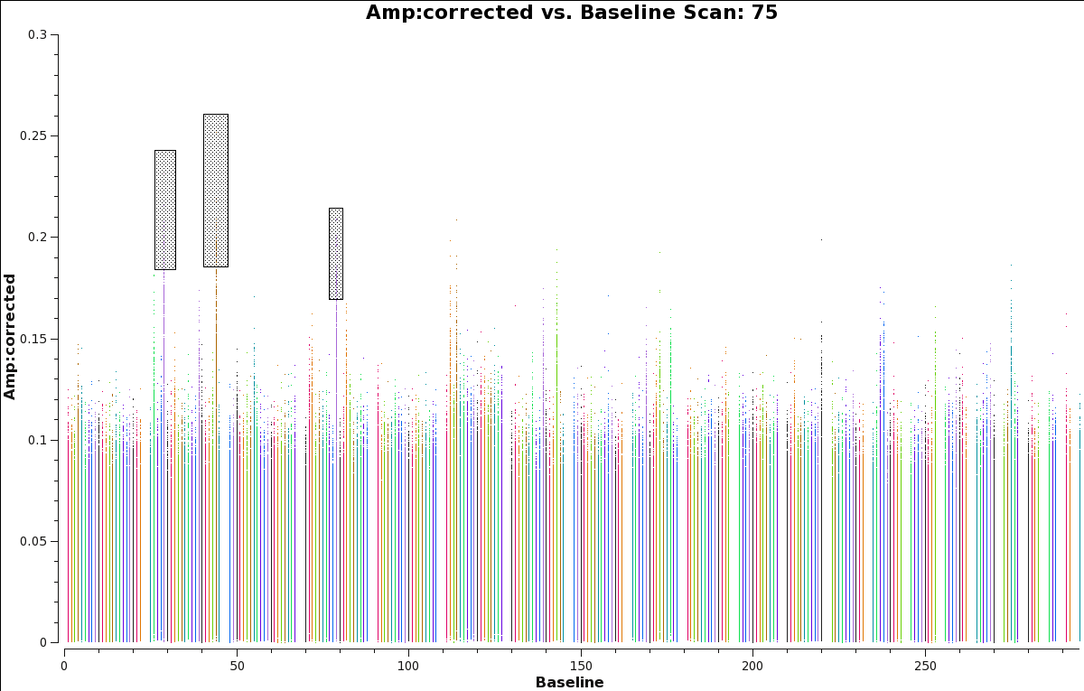
Amplitude vs. Baseline plot, which is used to try and identify baselines with high amplitudes for mutliple scans.
It appears that there are a several baselines which have consistently higher-amplitude than the others, indicating that they're probably contaminated by RFI (Figure 17).
Use the plotms tools to identify the baselines (see the section Preliminary Data Evaluation at the beginning of the guide). Iterate through to the different scans to verify that these higher amplitude correspond to the same baselines. We will flag several of them: ea04&ea16, ea02&ea08, and ea02&ea27.
# In CASA
flagdata(vis='SNR_G55_10s-hanning.ms', antenna='ea04&ea16', spw='1', flagbackup=False)
# In CASA
flagdata(vis='SNR_G55_10s-hanning.ms', antenna='ea02&ea27', spw='1', flagbackup=False)
# In CASA
flagdata(vis='SNR_G55_10s-hanning.ms', antenna='ea02&ea08', spw='1', flagbackup=False)
Interactive Flagging
To flag data interactively, we will use plotms to plot the corrected amplitude against uv-distance. We will be scanning for data points that look odd. A tutorial on flagging data interactively through plotms can be found on the Data flagging with plotms webpage. Please note that flagging data through plotms will not create a backup, so it's important to use the flagmanager before deciding to mark your regions for flagging purposes.
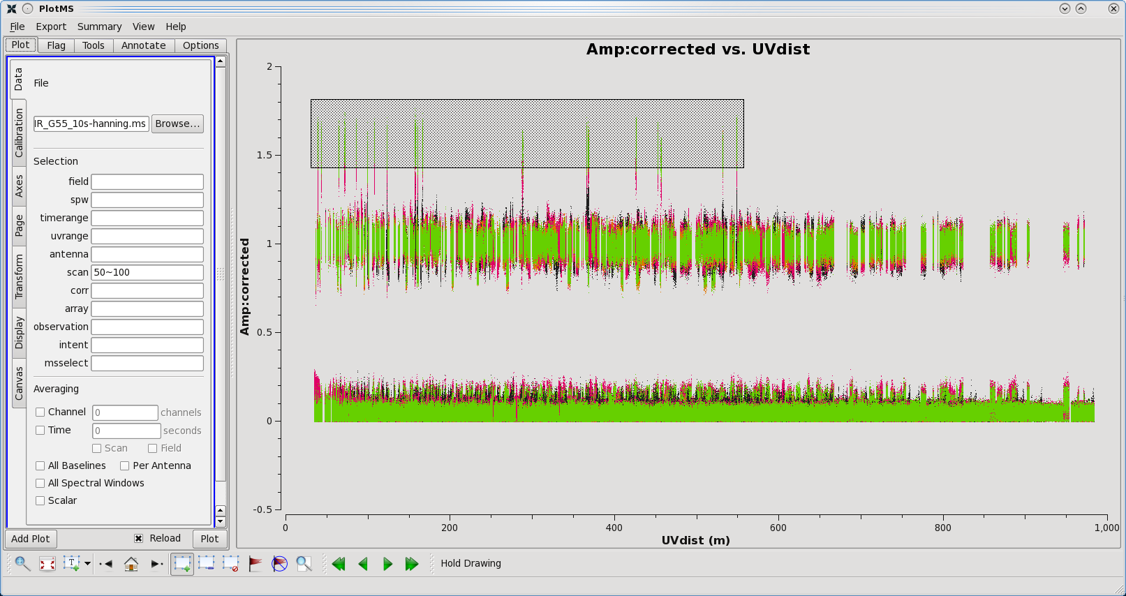
Amplitude vs. UV-Distance plot for scans 50-100. Outliers have been highlighted to show interactive flagging through plotms.
# In CASA
flagmanager(vis='SNR_G55_10s-hanning.ms', mode='save',
            versionname='before_interactive_flagging')
# In CASA
plotms(vis='SNR_G55_10s-hanning.ms', scan='50~100', xaxis='uvdist', yaxis='amp',
       ydatacolumn='corrected', coloraxis = 'spw')
Figure 18 shows some points in green that have higher amplitudes than the rest. We use the Mark Regions button (square with green plus sign) to highlight the region, and the Locate button (magnifying glass with white page) to give us information on the data points. We can now decide to flag all of the highlighted area by clicking on the Flag button (red flag).

Amplitude vs. UV-Distance plot for scans 50-100. Scans 87 and 88 have been flagged for ea16 via flagdata.
Flagging data interactively can be useful, but is discouraged. A more proper form of flagging would be to narrow your search on bad data points and use a flagging task to remove them. For example, after having located the region, the CASA logger will give you information on the data points. Notice that they all belong to scans 88 and 87. The scans also involve a baseline shared with ea16.
# In CASA
flagdata(vis='SNR_G55_10s-hanning.ms', scan='87,88', antenna='ea16', flagbackup=True)
# In CASA
plotms(vis='SNR_G55_10s-hanning.ms', scan='50~100', xaxis='uvdist', yaxis='amp',
       ydatacolumn='corrected', coloraxis = 'spw')
Re-plotting, we can see the image (Figure 19) looks better without scans 87 and 88 for ea16. Now would be a good time to play with the plotms parameters and look for more data to flag interactively. As a reminder, at the start of this guide we highlighted and located some of the worst sections with RFI. When reducing/flagging your data, it will prove helpful to review this information and revisit the most RFI affected spectral windows and channels.
Flagging Summary & Report
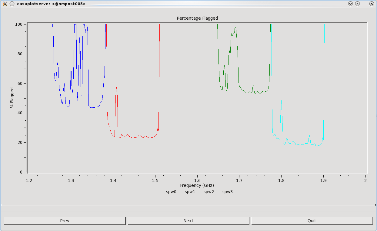
Total percentage of flagged data per spectral window.
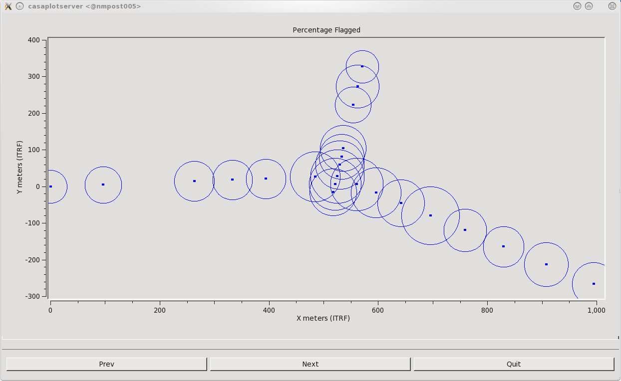
Total Percentage of data flagged from each antenna. A larger circle represents more flagged data for that antenna.
We will now run flagdata in summary mode to inspect how much total data has been flagged. We can also create a plot of the percentage of flagged data with respect to frequency by setting parameter display='report' (Figure 20). The report parameter will also create a plot of the antennas, with the circle size representing the percentage of flagged data per antenna (Figure 21). This can be viewed by clicking Next. One can also zoom in and out for a better view.
# In CASA
flagInfo = flagdata(vis='SNR_G55_10s-hanning.ms', mode='summary', action='calculate', display='report', spwchan=T)
# In CASA
print("\n %2.1f%% of G55.7+3.4, %2.1f%% of 3C147, and %2.1f%% of J1925+2106 are flagged. \n" %
     (100.0 * flagInfo['field']['G55.7+3.4']['flagged'] / flagInfo['field']['G55.7+3.4']['total'],
     100.0 * flagInfo['field']['0542+498=3C147']['flagged'] / flagInfo['field']['0542+498=3C147']['total'],
     100.0 * flagInfo['field']['J1925+2106']['flagged'] / flagInfo['field']['J1925+2106']['total']))
# In CASA
print("Spectral windows are flagged as follows:")

for spw in range(0,4):
     print("SPW %s: %2.1f%%" % (spw, 100.0 * flagInfo['spw'][str(spw)]['flagged'] / flagInfo['spw'][str(spw)]['total']))
As a result of the flagging we have removed over 40% of the data for G55.7+3.4 and, as expected, spectral windows 0 and 2 have the most flagged data.
In addition, we can inspect the CASA log, which will report the percentage of flagged data for:
1. per Spw/ per Channel
2. Each Antenna
3. Every Correlation (RR, RL, LL, LR)
4. Every Scan
5. Every spectral window