EVLA Continuum Tutorial 3C391-CASA4.5
This CASA Guide is for Version 4.5 of CASA. If you are using a later version of CASA and this is the most recent available guide, then you should be able to use most, if not all, of this casaguide, as we try to limit script breaking changes in CASA development.
Overview
This article describes the calibration and imaging of a multiple-pointing EVLA continuum dataset on the supernova remnant 3C 391. The data were taken in EVLA early science OSRO1 mode, with 128 MHz of bandwidth in each of two widely spaced spectral windows, centered at 4.6 and 7.5 GHz, and were set up for full polarization calibration.
Obtaining the Data
For the purposes of this tutorial, we have created a starting data set, upon which several initial processing steps have already been conducted. You may obtain the data set from here: http://casa.nrao.edu/Data/EVLA/3C391/3c391_ctm_mosaic_10s_spw0.ms.tgz (dataset size: 3.1GB)
If you wish to start from the very beginning, you may download the dataset from the NRAO Archive: TDEM0001_sb1218006_1.55310.33439732639
We are providing this starting data set, rather than the true initial data set for at least two reasons. First, many of these initial processing steps can be rather time consuming (> 1 hr). Second, while necessary, many of these steps are not fundamental to the calibration and imaging process, which is the focus of this tutorial. For completeness, however, here are the steps that were taken from the initial data set to produce the starting data set.
- The initial Science Data Model (SDM) file was converted into a measurement set.
- Basic data flagging was applied, to account for shadowing of the antennas. These data are from the D configuration, in which antennas are particularly susceptible to being blocked (shadowed) by other antennas in the array, depending upon the elevation of the source.
- The data were averaged from the initial 1-second correlator sample time to 10-second samples. In the D configuration, the fringe rate is relatively slow and time-average smearing is less of a concern.
- The data were acquired with two spectral windows (around 4.6 and 7.5 GHz). Because of disk space concerns on some machines, the focus will be on only one of the two spectral windows.
All of these steps can be done directly from the NRAO Archive's Download page, by selecting CASA MS as the download format (it's a good idea to also check the Create MS or SDM tar file box), checking the Apply flags generated during observing box, and setting Time Averaging to 10s.
Once the download is complete, unzip and unpack the file (within a working directory, which you will then run CASA):
# In a Terminal:
tar xzvf 3c391_ctm_mosaic_10s_spw0.ms.tgz
How to Use This CASA Guide
here are a number of possible ways to run CASA, described in more detail in Getting Started in CASA. In brief, there are at least three different ways to run CASA:
- Interactively examining task inputs. In this mode, one types taskname to load the task, inp to examine the inputs, and go once those inputs have been set to your satisfaction. Allowed inputs are shown in blue and bad inputs are colored red. The input parameters themselves are changed one by one, e.g., selectdata=T. Screenshots of the inputs to various tasks used in the data reduction below are provided, to illustrate which parameters need to be set. More detailed help can be obtained on any task by typing help taskname. Once a task is run, the set of inputs are stored and can be retrieved via tget taskname; subsequent runs will overwrite the previous tget file.
- Pseudo-interactively via task function calls. In this case, all of the desired inputs to a task are provided at once on the CASA command line. This tutorial is made up of such calls, which were developed by looking at the inputs for each task and deciding what needed to be changed from default values. For task function calls, only parameters that you want to be different from their defaults need to be set.
- Non-interactively via a script. A series of task function calls can be combined together into a script, and run from within CASA via execfile('scriptname.py'). This and other CASA Tutorial Guides have been designed to be extracted into a script via the script extractor by using the method described at the Extracting_scripts_from_these_tutorials page. Should you use the script generated by the script extractor for this CASA Guide, be aware that it will require some small amount of interaction related to the plotting, occasionally suggesting that you close the graphics window and hitting return in the terminal to proceed. It is in fact unnecessary to close the graphics windows (it is suggested that you do so purely to keep your desktop uncluttered).
If you are a relative novice or just new to CASA, it is strongly recommended to work through this tutorial by cutting and pasting the task function calls provided below after you have read all the associated explanations. Work at your own pace, look at the inputs to the tasks to see what other options exist, and read the help files. Later, when you are more comfortable, you might try to extract the script, modify it for your purposes, and begin to reduce other data.
The Observation
Before starting the calibration process, we want to get some basic information about the data set. To examine the observing conditions during the observing run, and to find out any known problems with the data, download the observer log. Simply fill in the known observing date (in our case 2010-Apr-24) as both the Start and Stop date, and click on the Show Logs button. The relevant log is labeled with the project code, TDEM0001, and can be downloaded as a PDF file. From this, we find the following:
Information from observing log:
There is no C-band receivers on ea13
Antenna ea06 is out of the array
Antenna ea15 has some corrupted data
Antennas ea10, ea12, ea22 do not have good baseline positions
Gusty winds, mixed clouds, API rms up to 11.5.
Before beginning our data reduction, we must start CASA. If you have not used CASA before, some helpful tips are available on the Getting Started in CASA page.
Once you have CASA up and running in the directory containing the data, then start your data reduction by getting some basic information about the data. The task listobs can be used to get a listing of the individual scans comprising the observation, the frequency setup, source list, and antenna locations.
# In CASA
listobs(vis='3c391_ctm_mosaic_10s_spw0.ms')
One will note that there are nine sources observed. Here the various sources are introduced briefly, with more detail contained in the sections below in which they are used.
- J1331+3030 = 3C 286, which will later serve as a calibrator for the visibility amplitudes, i.e., it is assumed to have a precisely known flux density; the spectral bandpass; and the polarization position angle;
- J1822-0938, which will serve as a calibrator for the visibility phases;
- J0319+4130 = 3C 84, which will serve as a polarization calibrator; and
- 3C391 C1–C7, which are 7 fields centered on and surrounding the supernova remnant.
This observation was set up as a 7-pointing mosaic because the supernova remnant is so large that it essentially fills the primary beam.
##########################################
##### Begin Task: listobs #####
listobs(vis="3c391_ctm_mosaic_10s_spw0.ms",selectdata=True,spw="",field="",antenna="",
uvrange="",timerange="",correlation="",scan="",intent="",
feed="",array="",observation="",verbose=True,listfile="",
listunfl=False,cachesize=50,overwrite=False)
================================================================================
MeasurementSet Name: 3c391_ctm_mosaic_10s_spw0.ms MS Version 2
================================================================================
Observer: Dr. James Miller-Jones Project: T.B.D.
Observation: EVLA
Data records: 845379 Total integration time = 28681.5 seconds
Observed from 24-Apr-2010/08:02:10.0 to 24-Apr-2010/16:00:11.5 (UTC)
ObservationID = 0 ArrayID = 0
Date Timerange (UTC) Scan FldId FieldName nRows SpwIds Average Interval(s) ScanIntent
24-Apr-2010/08:02:10.0 - 08:02:30.0 1 0 J1331+3030 650 [0] [10]
08:02:20.0 - 08:09:30.0 2 0 J1331+3030 13975 [0] [10]
08:09:20.0 - 08:16:28.0 3 0 J1331+3030 13975 [0] [10]
08:19:38.0 - 08:24:26.5 4 1 J1822-0938 7035 [0] [10]
08:24:48.0 - 08:29:48.0 5 2 3C391 C1 7590 [0] [10]
08:29:38.0 - 08:34:48.0 6 3 3C391 C2 7821 [0] [10]
08:34:38.0 - 08:39:48.0 7 4 3C391 C3 7821 [0] [10]
08:39:38.0 - 08:44:48.0 8 5 3C391 C4 7821 [0] [10]
08:44:38.0 - 08:49:48.0 9 6 3C391 C5 7843 [0] [10]
08:49:38.0 - 08:54:48.0 10 7 3C391 C6 7843 [0] [10]
08:54:38.0 - 08:59:43.5 11 8 3C391 C7 7843 [0] [10]
09:00:03.0 - 09:01:31.0 12 1 J1822-0938 2925 [0] [10]
09:01:52.0 - 09:06:52.0 13 2 3C391 C1 7941 [0] [10]
09:06:42.0 - 09:11:52.0 14 3 3C391 C2 9801 [0] [10]
09:11:42.0 - 09:16:52.0 15 4 3C391 C3 10075 [0] [10]
09:16:42.0 - 09:21:52.0 16 5 3C391 C4 10050 [0] [10]
09:21:42.0 - 09:26:52.0 17 6 3C391 C5 10075 [0] [10]
09:26:42.0 - 09:31:52.0 18 7 3C391 C6 10075 [0] [10]
09:31:42.0 - 09:36:47.5 19 8 3C391 C7 10075 [0] [10]
09:37:07.0 - 09:38:35.0 20 1 J1822-0938 2900 [0] [10]
09:38:57.0 - 09:43:57.0 21 2 3C391 C1 9700 [0] [10]
09:43:47.0 - 09:48:57.0 22 3 3C391 C2 10050 [0] [10]
09:48:47.0 - 09:53:57.0 23 4 3C391 C3 10075 [0] [10]
09:53:47.0 - 09:58:57.0 24 5 3C391 C4 10075 [0] [10]
09:58:47.0 - 10:03:57.0 25 6 3C391 C5 10075 [0] [10]
10:03:47.0 - 10:08:57.0 26 7 3C391 C6 10075 [0] [10]
10:08:47.0 - 10:13:47.0 27 8 3C391 C7 9750 [0] [10]
10:14:12.0 - 10:15:39.5 28 1 J1822-0938 2925 [0] [10]
10:16:01.0 - 10:21:01.0 29 2 3C391 C1 9000 [0] [10]
10:20:51.0 - 10:26:01.0 30 3 3C391 C2 10050 [0] [10]
10:25:51.0 - 10:31:01.0 31 4 3C391 C3 10075 [0] [10]
10:30:51.0 - 10:36:01.0 32 5 3C391 C4 10075 [0] [10]
10:35:51.0 - 10:41:01.0 33 6 3C391 C5 10075 [0] [10]
10:40:51.0 - 10:46:01.0 34 7 3C391 C6 10075 [0] [10]
10:45:51.0 - 10:50:51.0 35 8 3C391 C7 9750 [0] [10]
10:51:15.0 - 10:52:42.5 36 1 J1822-0938 2925 [0] [10]
10:55:14.0 - 10:57:42.0 37 0 J1331+3030 3364 [0] [10]
11:00:13.0 - 11:02:41.0 38 1 J1822-0938 3883 [0] [10]
11:03:03.0 - 11:08:03.0 39 2 3C391 C1 9750 [0] [10]
11:07:53.0 - 11:12:53.0 40 3 3C391 C2 9725 [0] [10]
11:12:43.0 - 11:17:43.0 41 4 3C391 C3 9750 [0] [10]
11:17:33.0 - 11:22:33.0 42 5 3C391 C4 9750 [0] [10]
11:22:23.0 - 11:27:23.0 43 6 3C391 C5 9750 [0] [10]
11:27:13.0 - 11:32:13.0 44 7 3C391 C6 9750 [0] [10]
11:32:03.0 - 11:36:53.0 45 8 3C391 C7 9425 [0] [10]
11:37:21.0 - 11:38:47.0 46 1 J1822-0938 2700 [0] [10]
11:39:11.0 - 11:44:11.0 47 2 3C391 C1 9750 [0] [10]
11:44:01.0 - 11:49:01.0 48 3 3C391 C2 9700 [0] [10]
11:48:51.0 - 11:53:41.0 49 4 3C391 C3 8355 [0] [10]
11:53:41.0 - 11:58:31.0 50 5 3C391 C4 9425 [0] [10]
11:58:21.0 - 12:03:21.0 51 6 3C391 C5 9725 [0] [10]
12:03:11.0 - 12:08:11.0 52 7 3C391 C6 9701 [0] [10]
12:08:01.0 - 12:12:59.0 53 8 3C391 C7 9725 [0] [10]
12:13:29.0 - 12:14:48.0 54 1 J1822-0938 2600 [0] [10]
12:15:18.0 - 12:20:08.0 55 2 3C391 C1 9425 [0] [10]
12:19:58.0 - 12:24:58.0 56 3 3C391 C2 9750 [0] [10]
12:24:48.0 - 12:29:48.0 57 4 3C391 C3 9750 [0] [10]
12:29:38.0 - 12:34:38.0 58 5 3C391 C4 9725 [0] [10]
12:34:28.0 - 12:39:28.0 59 6 3C391 C5 9725 [0] [10]
12:39:18.0 - 12:44:18.0 60 7 3C391 C6 9750 [0] [10]
12:44:08.0 - 12:49:04.5 61 8 3C391 C7 9750 [0] [10]
12:49:35.0 - 12:50:53.0 62 1 J1822-0938 2600 [0] [10]
12:51:24.0 - 12:56:14.0 63 2 3C391 C1 9425 [0] [10]
12:56:04.0 - 13:01:04.0 64 3 3C391 C2 9000 [0] [10]
13:00:54.0 - 13:05:54.0 65 4 3C391 C3 9750 [0] [10]
13:05:44.0 - 13:10:44.0 66 5 3C391 C4 9750 [0] [10]
13:10:34.0 - 13:15:34.0 67 6 3C391 C5 9725 [0] [10]
13:15:24.0 - 13:20:24.0 68 7 3C391 C6 9750 [0] [10]
13:20:14.0 - 13:25:10.0 69 8 3C391 C7 9000 [0] [10]
13:25:40.0 - 13:26:57.5 70 1 J1822-0938 2600 [0] [10]
13:27:28.0 - 13:32:18.0 71 2 3C391 C1 9425 [0] [10]
13:32:08.0 - 13:37:08.0 72 3 3C391 C2 9750 [0] [10]
13:36:58.0 - 13:41:58.0 73 4 3C391 C3 9750 [0] [10]
13:41:48.0 - 13:46:48.0 74 5 3C391 C4 9750 [0] [10]
13:46:38.0 - 13:51:38.0 75 6 3C391 C5 9725 [0] [10]
13:51:28.0 - 13:56:28.0 76 7 3C391 C6 9750 [0] [10]
13:56:18.0 - 14:01:14.0 77 8 3C391 C7 9750 [0] [10]
14:01:44.0 - 14:03:01.5 78 1 J1822-0938 2024 [0] [10]
14:03:33.0 - 14:08:23.0 79 2 3C391 C1 8900 [0] [10]
14:08:13.0 - 14:13:13.0 80 3 3C391 C2 9750 [0] [10]
14:13:03.0 - 14:18:03.0 81 4 3C391 C3 9750 [0] [10]
14:17:53.0 - 14:22:53.0 82 5 3C391 C4 9350 [0] [10]
14:22:43.0 - 14:27:43.0 83 6 3C391 C5 9000 [0] [10]
14:27:33.0 - 14:32:33.0 84 7 3C391 C6 8595 [0] [10]
14:32:23.0 - 14:37:18.5 85 8 3C391 C7 7590 [0] [10]
14:37:48.0 - 14:39:05.5 86 1 J1822-0938 1848 [0] [10]
14:39:36.0 - 14:44:26.0 87 2 3C391 C1 7337 [0] [10]
14:44:16.0 - 14:49:16.0 88 3 3C391 C2 7568 [0] [10]
14:49:06.0 - 14:54:06.0 89 4 3C391 C3 7590 [0] [10]
14:53:56.0 - 14:58:56.0 90 5 3C391 C4 7527 [0] [10]
14:58:46.0 - 15:03:46.0 91 6 3C391 C5 7568 [0] [10]
15:03:36.0 - 15:08:36.0 92 7 3C391 C6 7590 [0] [10]
15:08:26.0 - 15:13:22.0 93 8 3C391 C7 7590 [0] [10]
15:13:51.0 - 15:15:09.0 94 1 J1822-0938 1680 [0] [10]
15:15:40.0 - 15:20:30.0 95 2 3C391 C1 7337 [0] [10]
15:20:20.0 - 15:25:20.0 96 3 3C391 C2 7568 [0] [10]
15:25:10.0 - 15:30:10.0 97 4 3C391 C3 7590 [0] [10]
15:30:00.0 - 15:35:00.0 98 5 3C391 C4 7564 [0] [10]
15:34:50.0 - 15:39:50.0 99 6 3C391 C5 7260 [0] [10]
15:39:40.0 - 15:44:40.0 100 7 3C391 C6 6930 [0] [10]
15:44:30.0 - 15:49:26.0 101 8 3C391 C7 6930 [0] [10]
15:49:55.0 - 15:51:13.5 102 1 J1822-0938 1088 [0] [10]
15:54:52.0 - 16:00:11.5 103 9 J0319+4130 8768 [0] [10]
(nRows = Total number of rows per scan)
Fields: 10
ID Code Name RA Decl Epoch SrcId nRows
0 N J1331+3030 13:31:08.287984 +30.30.32.95886 J2000 0 31964
1 J J1822-0938 18:22:28.704200 -09.38.56.83501 J2000 1 39733
2 NONE 3C391 C1 18:49:24.244000 -00.55.40.58001 J2000 2 105580
3 NONE 3C391 C2 18:49:29.149001 -00.57.48.00001 J2000 3 110533
4 NONE 3C391 C3 18:49:19.339000 -00.57.48.00001 J2000 4 110331
5 NONE 3C391 C4 18:49:14.434001 -00.55.40.58001 J2000 5 110862
6 NONE 3C391 C5 18:49:19.339000 -00.53.33.16000 J2000 6 110546
7 NONE 3C391 C6 18:49:29.149001 -00.53.33.16000 J2000 7 109884
8 NONE 3C391 C7 18:49:34.054000 -00.55.40.58001 J2000 8 107178
9 Z J0319+4130 03:19:48.160102 +41.30.42.10305 J2000 9 8768
Spectral Windows: (1 unique spectral windows and 1 unique polarization setups)
SpwID Name #Chans Frame Ch0(MHz) ChanWid(kHz) TotBW(kHz) CtrFreq(MHz) Corrs
0 Subband:0 64 TOPO 4536.000 2000.000 128000.0 4599.0000 RR RL LR LL
Sources: 10
ID Name SpwId RestFreq(MHz) SysVel(km/s)
0 J1331+3030 0 - -
1 J1822-0938 0 - -
2 3C391 C1 0 - -
3 3C391 C2 0 - -
4 3C391 C3 0 - -
5 3C391 C4 0 - -
6 3C391 C5 0 - -
7 3C391 C6 0 - -
8 3C391 C7 0 - -
9 J0319+4130 0 - -
Antennas: 26:
ID Name Station Diam. Long. Lat. Offset from array center (m) ITRF Geocentric coordinates (m)
East North Elevation x y z
0 ea01 W09 25.0 m -107.37.25.2 +33.53.51.0 -521.9407 -332.7782 -1.1977 -1601710.017000 -5042006.928200 3554602.355600
1 ea02 E02 25.0 m -107.37.04.4 +33.54.01.1 9.8247 -20.4292 -2.7808 -1601150.059500 -5042000.619800 3554860.729400
2 ea03 E09 25.0 m -107.36.45.1 +33.53.53.6 506.0591 -251.8666 -3.5832 -1600715.948000 -5042273.187000 3554668.184500
3 ea04 W01 25.0 m -107.37.05.9 +33.54.00.5 -27.3562 -41.3030 -2.7418 -1601189.030140 -5042000.493300 3554843.425700
4 ea05 W08 25.0 m -107.37.21.6 +33.53.53.0 -432.1158 -272.1493 -1.5032 -1601614.091000 -5042001.655700 3554652.509300
5 ea07 N06 25.0 m -107.37.06.9 +33.54.10.3 -54.0667 263.8720 -4.2292 -1601162.593200 -5041829.000000 3555095.890500
6 ea08 N01 25.0 m -107.37.06.0 +33.54.01.8 -30.8810 -1.4664 -2.8597 -1601185.634945 -5041978.156586 3554876.424700
7 ea09 E06 25.0 m -107.36.55.6 +33.53.57.7 236.9058 -126.3369 -2.4443 -1600951.588000 -5042125.911000 3554773.012300
8 ea11 E04 25.0 m -107.37.00.8 +33.53.59.7 102.8046 -63.7684 -2.6412 -1601068.791200 -5042051.910200 3554824.835300
9 ea12 E08 25.0 m -107.36.48.9 +33.53.55.1 407.8394 -206.0057 -3.2252 -1600801.916000 -5042219.371000 3554706.449900
10 ea13 N07 25.0 m -107.37.07.2 +33.54.12.9 -61.1040 344.2335 -4.6144 -1601155.635800 -5041783.843000 3555162.374100
11 ea14 E05 25.0 m -107.36.58.4 +33.53.58.8 164.9788 -92.8032 -2.5268 -1601014.462000 -5042086.252000 3554800.799800
12 ea15 W06 25.0 m -107.37.15.6 +33.53.56.4 -275.8288 -166.7451 -2.0590 -1601447.198000 -5041992.502500 3554739.687600
13 ea16 W02 25.0 m -107.37.07.5 +33.54.00.9 -67.9687 -26.5614 -2.7175 -1601225.255200 -5041980.383590 3554855.675000
14 ea17 W07 25.0 m -107.37.18.4 +33.53.54.8 -349.9866 -216.7507 -1.7978 -1601526.386100 -5041996.840100 3554698.327400
15 ea18 N09 25.0 m -107.37.07.8 +33.54.19.0 -77.4352 530.6274 -5.5867 -1601139.485500 -5041679.036000 3555316.532800
16 ea19 W04 25.0 m -107.37.10.8 +33.53.59.1 -152.8599 -83.8054 -2.4614 -1601315.893000 -5041985.320170 3554808.304600
17 ea20 N05 25.0 m -107.37.06.7 +33.54.08.0 -47.8454 192.6015 -3.8723 -1601168.786100 -5041869.054000 3555036.936000
18 ea21 E01 25.0 m -107.37.05.7 +33.53.59.2 -23.8638 -81.1510 -2.5851 -1601192.467800 -5042022.856800 3554810.438800
19 ea22 N04 25.0 m -107.37.06.5 +33.54.06.1 -42.5986 132.8623 -3.5431 -1601173.953700 -5041902.660400 3554987.536500
20 ea23 E07 25.0 m -107.36.52.4 +33.53.56.5 318.0523 -164.1848 -2.6960 -1600880.570000 -5042170.388000 3554741.457400
21 ea24 W05 25.0 m -107.37.13.0 +33.53.57.8 -210.0944 -122.3885 -2.2581 -1601377.008000 -5041988.665500 3554776.393400
22 ea25 N02 25.0 m -107.37.06.2 +33.54.03.5 -35.6245 53.1806 -3.1345 -1601180.861480 -5041947.453400 3554921.628700
23 ea26 W03 25.0 m -107.37.08.9 +33.54.00.1 -105.3429 -51.7191 -2.6054 -1601265.151700 -5041982.533050 3554834.856300
24 ea27 E03 25.0 m -107.37.02.8 +33.54.00.5 50.6647 -39.4832 -2.7249 -1601114.365500 -5042023.153700 3554844.945600
25 ea28 N08 25.0 m -107.37.07.5 +33.54.15.8 -68.9057 433.1889 -5.0602 -1601147.940400 -5041733.837000 3555235.956000
##### End Task: listobs #####
##########################################
Note that the antenna IDs (which are numbered sequentially up to the total number of antennas in the array; 0 through 25 in this instance) do not correspond to the actual antenna names (ea01 through ea28; these numbers correspond to those painted on the side of the dishes). The antennas can be referenced using either convention; antenna='22' would correspond to ea25, whereas antenna='ea22' would correspond to ea22. Note that the antenna numbers in the observer log correspond to the actual antenna names, i.e., the 'ea??' numbers given in listobs.
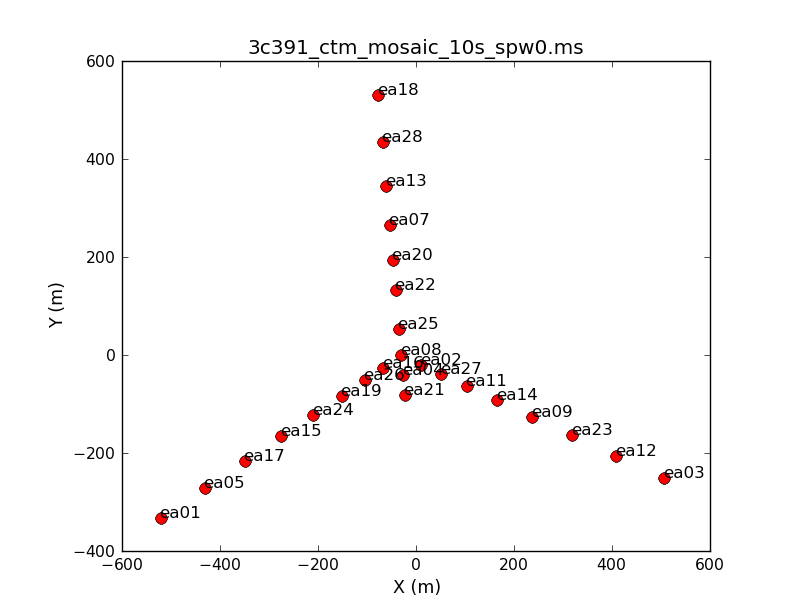
Both to get a sense of the array, as well as identify an antenna for later use in calibration, use the task plotants (see Figure 1). In general, for calibration purposes, one would like to select an antenna that is close to the center of the array (and that is not listed in the operator's log as having had problems!).
# In CASA
plotants(vis='3c391_ctm_mosaic_10s_spw0.ms',figfile='plotants_3c391_antenna_layout.png')
clearstat() # This removes the table lock generated by plotants in script mode
Examining and Editing the Data
It is always a good idea, particularly with a new system like the JVLA, to examine the data. Moreover, from the observer's log, we already know that one antenna will need to be flagged because it does not have a C-band receiver. Start by flagging data known to be bad, then examine the data.
In the scheduling block configuration, it is common to insert a dummy scan as the first scan. From the listobs output above, one may have noticed that the first scan is less than 1 minute long. This first scan can safely be flagged.
# In CASA
flagdata(vis='3c391_ctm_mosaic_10s_spw0.ms', flagbackup=T,
         mode='manual', scan='1')
- flagbackup=T : A comment is warranted on the setting of flagbackup (here set to T or True). If set to True, flagdata will save a copy of the existing set of flags before entering any new flags. The setting of flagbackup is therefore a matter of some taste. You could choose not to save any flags or only save major flags, or you could save every flag.
- mode='manualflag' : Specific data are going to be selected to be edited.
- scan='1' : is chosen to select only the first scan. Note that scan expects an entry in the form of a string (scan=1 would generate an error).
If satisfied with the inputs, run this task. The initial display in the logger will include
##########################################
##### Begin Task: flagdata           #####
.
.
.
.
Backup original flags before applying new flags
Table type is Measurement Set
 	Creating new backup flag file called flagdata_1
Table type is Measurement Set
Manual mode is active
Parsing the parameters for the manual mode
Initializing the agents
Manual	 autocorr is 0
There are 1 valid agents in list
Running the agentflagger tool
------------------------------------------------------------------------------------
Chunk = 1 [progress: 100%], Observation = 0, Array = 0, Scan = 1, Field = 0 (J1331+3030), Spw = 0, Channels = 64, Corrs = [ RR RL LR LL ], Total Rows = 650
Manual	=> Data flagged so far 100%
====================================================================================
=> Percentage of data flagged in table selection: 100%
=> Writing flags to the MS
##### End Task: flagdata             #####
##########################################
which indicates that, among other things, the flags that existed in the data set prior to this run will be saved to another file called flagdata_1. Should you ever desire to revert to the data prior to this run, the task flagmanager could be used. Also note that the values of all the task parameters (explicit or hidden) are given at the start of the task listing.
From the observer's log, we know that antenna ea13 does not have a C-band receiver and antenna ea15 had some corrupted data, so they should be flagged as well. The parameters are similar as before.
# In CASA
flagdata(vis='3c391_ctm_mosaic_10s_spw0.ms', flagbackup=T, mode='manual',
         antenna='ea13,ea15')
- antenna='ea13,ea15' : Once again, this parameter requires a string input. Remember that antenna='ea13' and 'antenna='13' are not the same antenna. (See the discussion after our call to listobs above.)
Finally, it is common for the array to require a small amount of time to settle down at the start of a scan. Consequently, it has become standard practice to flag the initial samples from the start of each scan.
# In CASA
flagdata(vis='3c391_ctm_mosaic_10s_spw0.ms', mode='quack',
         quackinterval=10.0, quackmode='beg')
- mode='quack' : Quack is another mode in which the same edit will be applied to all scans for all baselines.
- quackmode='beg' : In this case, data from the start of each scan will be flagged. Other options include flagging data at the end of the scan.
- quackinterval=10 : In this data set, the sampling time is 10 seconds, so this choice flags the first sample from all scans on all baselines.
Having now done some basic editing of the data, based in part on a priori information, it is time to look at the data to determine if there are any other obvious problems. One task to examine the data themselves is plotms.
# In CASA
clearstat() # This removes any existing table locks generated by flagdata
plotms(vis='3c391_ctm_mosaic_10s_spw0.ms', selectdata=True, field='0')
- selectdata=T : One can choose to plot only subsets of the data.
- field='0' : The entire dataset is rather large, and different sources have very different amplitudes, so it is advisable to start by loading a subset of the data. You can later loop through the different fields (i.e. sources) and spectral windows using the GUI interface.
In this case, many other values have been left to defaults, but it is possible to select them from within the plotms GUI.
Task plotms should produce a GUI, with the default view being to show the visibility amplitude as a function of time. Figure 2 shows the result of running plotms without the field selection discussed above (using field=' ' ).
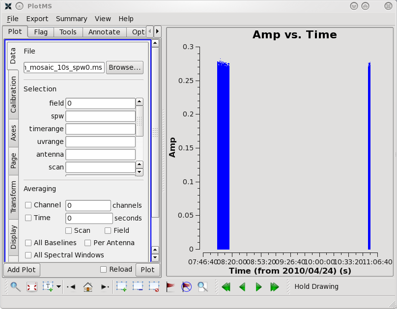
Task plotms allows one to select and view the data in many ways. Across the top of the left panel are a set of tabs labeled Plots, Flagging, Tools, Annotator, and Options. The option under the Flagging tab is to Extend flags; thus, even though plotms was started with extendflag=F, if you decide that it does make sense to extend the flags, you can do so here.
In the default view, the Plots tab is visible, and there are a number of tabs running down the side of the left hand panel, including Data, Axes, Trans, Cache, Display, Canvas, and Export. These allow you to make changes without having to re-launch plotms. Even if plotms was started with plotfile=' ' , you can save a copy of the plot by selecting the Export tab and entering a file name.
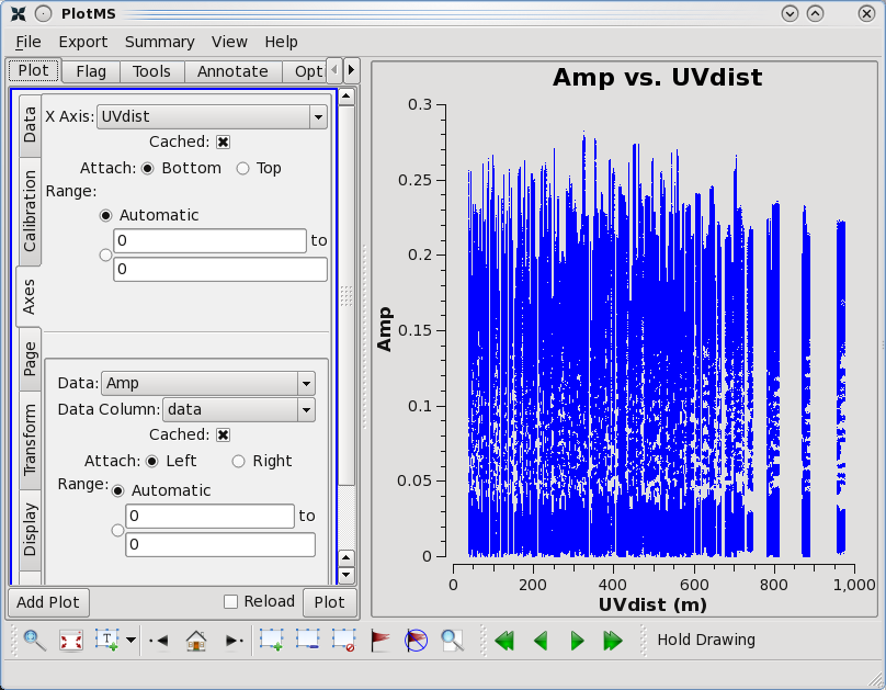
You should spend several minutes displaying the data in various formats. For instance, you could select the Data tab and specify field 0 (source J1331+3030, a.k.a. 3C 286) to display data associated with the amplitude calibrator, then select the Axes tab and change the X-axis to be UVDist (baseline length in meters), and plot the data. The result should be similar to Figure 3A. The amplitude distribution is relatively constant as a function of u–v distance or baseline length (i.e., [math]\displaystyle{ \sqrt{u^2+v^2} }[/math] ). You should recognize that a relatively constant visibility amplitude, as a function of baseline length, means that the source is very nearly a point source. (The Fourier transform of a constant is a delta function, a.k.a., a point source.)
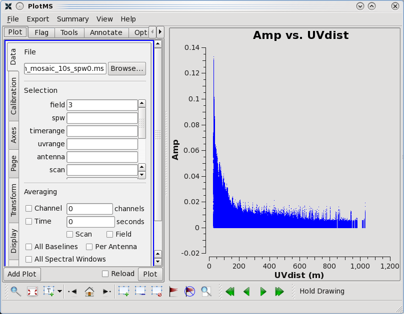
By contrast, if you select field 3 (one of the 3C 391 fields) in the Data tab and plot these data, one sees a visibility function that falls rapidly with increasing baseline length (see Figure 3B). Such a visibility function indicates a highly resolved source. By noting the baseline length at which the visibility function falls to some fiducial value (e.g., 1/2 of its peak value), a rough estimate of the angular scale of the source can be obtained. (Angular scale [in radians] ~ 1/baseline [in wavelengths]. To plot baseline length in wavelengths rather than meters, one needs to select UVwave as the X-axis in the plotms GUI.)
At this stage in the data reduction process, the general data editing and examination strategy is to focus is on the calibrators. The reduction strategy is to determine various corrections from the calibrators, then apply these correction factors to the science data. The 3C 286 data look relatively clean in that there are no wildly egregious data (e.g., amplitudes that are 100,000x larger than the rest of the data). One may notice that there are antenna-to-antenna variations (under the Display tab select Colorize by Antenna1). These antenna-to-antenna variations are acceptable, that's what calibration will help determine.
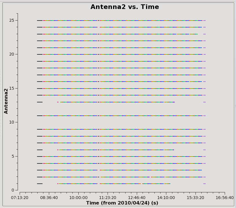
One final useful plot we will make is a datastream plot of the antenna2 in a baseline for the data versus ea01. This shows, assuming that ea01 is in the entire observation, when various antennas drop out.
# In CASA
plotms(vis='3c391_ctm_mosaic_10s_spw0.ms',field='',correlation='RR,LL',
       timerange='',antenna='ea01',spw='0:31',
       xaxis='time',yaxis='antenna2',
       plotrange=[-1,-1,0,26],coloraxis='field')
From this display (see Figure 4), you can see that antenna 3 (ea04) is missing the last scan on 3C84 (which will have some implications later on); antennas 1,6, and 13 (ea02,ea08, and ea16) have some missing blocks of time in the middle of the run; and 23 (ea26) is missing a scan or two near the end.
Calibrating the Data
It is now time to begin calibrating the data. The general data reduction strategy is to derive a series of scaling factors or corrections from the calibrators, which are then collectively applied to the science data. For more discussion of the philosophy, strategy, and implementation of calibration of synthesis data within CASA, see Synthesis Calibration in the CASA Reference Manual.
Recall that the observed visibility [math]\displaystyle{ V^{\prime} }[/math] between two antennas [math]\displaystyle{ (i,j) }[/math] is related to the true visibility [math]\displaystyle{ V }[/math] by:
[math]\displaystyle{ V^{\prime}_{i,j}(u,v,f) = b_{ij}(t)\,[B_i(f,t) B^{*}_j(f,t)]\,g_i(t) g_j(t)\,V_{i,j}(u,v,f)\,e^{i [\theta_i(t) - \theta_j(t)]} }[/math]
Here, for generality, we show the visibility as a function of frequency [math]\displaystyle{ f }[/math] and spatial wave numbers [math]\displaystyle{ u }[/math] and [math]\displaystyle{ v }[/math]. The other terms are:
- [math]\displaystyle{ g_i }[/math] and [math]\displaystyle{ \theta_i }[/math] are the amplitude and phase portions of what is commonly termed the complex gain. They are shown separately here because they are usually determined separately. For completeness, these are shown as a function of time [math]\displaystyle{ t }[/math] to indicate that they can change with temperature, atmospheric conditions, etc.
- [math]\displaystyle{ B_i }[/math] is the complex bandpass, the instrumental response as a function of frequency, [math]\displaystyle{ f }[/math]. As shown here, the bandpass may also vary as a function of time.
- [math]\displaystyle{ b(t) }[/math] is the often-neglected baseline term. It can be important to include for the highest dynamic range images or shortly after a configuration change at the JVLA, when antenna positions may not be known well.
Strictly, the equation above is a simplification of a more general measurement equation formalism, but it is a useful simplification in many cases.
A priori Antenna Position Corrections
As mentioned in the observing log above, antennas ea10, ea12, and ea22 do not have good baseline positions. Antenna ea10 was not in the array, but, for the other two antennas, any improved baseline positions need to be incorporated. The importance of this step is that the visibility function is a function of [math]\displaystyle{ u }[/math] and [math]\displaystyle{ v }[/math]. If the baseline positions are incorrect, then [math]\displaystyle{ u }[/math] and [math]\displaystyle{ v }[/math] will be calculated incorrectly and there will be errors in the image. These corrections could also be determined later by a baseline-based calibration incorporating the [math]\displaystyle{ b_{ij} }[/math] term from the equation above, but since they are known a priori it makes sense to incorporate them now.
The calculations are inserted via gencal which, since CASA 3.4, allows automated lookup of the corrections. To see how to calculate corrections manually, go to the EVLA/VLA Baseline Corrections site.
# In CASA
gencal(vis='3c391_ctm_mosaic_10s_spw0.ms',caltable='3c391_ctm_mosaic_10s_spw0.antpos',caltype='antpos')
In the logger you can see the corrections reported:
##########################################
##### Begin Task: gencal             #####
gencal(vis="3c391_ctm_mosaic_10s_spw0.ms",caltable="3c391_ctm_mosaic_10s_spw0.antpos",caltype="antpos",infile="",spw="",
        antenna="",pol="",parameter=[])
Opening MS: 3c391_ctm_mosaic_10s_spw0.ms for calibration.
Initializing nominal selection to the whole MS.
Determine antenna position offests from the baseline correction database
offsets for antenna ea01 :  0.00000   0.00300   0.00000
offsets for antenna ea02 : -0.00080   0.00000   0.00000
offsets for antenna ea03 : -0.00280   0.00000   0.00000
offsets for antenna ea05 :  0.00000   0.00280   0.00000
offsets for antenna ea11 :  0.00090   0.00000   0.00000
offsets for antenna ea12 : -0.01000   0.00450  -0.00170
offsets for antenna ea13 :  0.00000  -0.00080   0.00000
offsets for antenna ea17 : -0.00120   0.00000   0.00000
offsets for antenna ea18 :  0.00040  -0.00080   0.00040
offsets for antenna ea22 : -0.02570   0.00270  -0.01900
offsets for antenna ea23 : -0.00140   0.00000   0.00000
offsets for antenna ea24 : -0.00150   0.00000   0.00000
offsets for antenna ea26 : -0.00190   0.00000   0.00210
offsets for antenna ea27 :  0.00000   0.00190  -0.00160
Beginning specifycal-----------------------
Creating KAntPos Jones table from specified parameters.
Writing solutions to table: 3c391_ctm_mosaic_10s_spw0.antpos
##### End Task: gencal               #####
##########################################
This corresponds to what is found in the database for 2010:
;                2010 BASELINE CORRECTIONS IN METERS
;ANT
;MOVED OBSDATE   Put_In_ MC(IAT)  ANT  PAD    Bx      By      Bz
;
JAN27   FEB12     FEB21  01:57    11   E04  0.0000  0.0000  0.0000
JAN27   FEB12     FEB21  01:57    26   W03 -0.0170  0.0204  0.0041
MAR24   MAR25     MAR26  18:28    17   W07 -0.0061 -0.0069 -0.0055
APR21   MAY02     MAY04  23:25    12   E08 -0.0072  0.0045 -0.0017
MAR09   MAY02     MAY04  23:25    22   N04 -0.0220  0.0040 -0.0190
JUN08   JUN20     JUN22  03:00    10   N03  0.0046 -0.0196  0.0090
        JUL17     JUL18  21:44     1   W09  0.0000  0.0030  0.0000
        JUL17     JUL18  21:44     2   E02 -0.0008  0.0000  0.0000
        JUL17     JUL18  21:44     3   E09 -0.0028  0.0000  0.0000
        JUL17     JUL18  21:44     5   W08  0.0000  0.0028  0.0000
JUL01   JUL17     JUL18  21:44     6   N06  0.0022  0.0010  0.0059
        JUL17     JUL18  21:44    10   N03  0.0008  0.0030 -0.0014
        JUL17     JUL18  21:44    11   E04  0.0009  0.0000  0.0000
        JUL17     JUL18  21:44    12   E08 -0.0028  0.0000  0.0000
        JUL17     JUL18  21:44    13   N07  0.0000 -0.0008  0.0000
        JUL17     JUL18  21:44    17   W07 -0.0012  0.0000  0.0000
        JUL17     JUL18  21:44    18   N09  0.0004 -0.0008  0.0004
        JUL17     JUL18  21:44    22   N04 -0.0037 -0.0013  0.0000
        JUL17     JUL18  21:44    23   E07 -0.0014  0.0000  0.0000
        JUL17     JUL18  21:44    24   W05 -0.0015  0.0000  0.0000
        JUL17     JUL18  21:44    26   W03 -0.0019  0.0000  0.0021
        JUL17     JUL18  21:44    27   E03  0.0000  0.0019 -0.0016
AUG05   SEP15     SEP16  00:11    07   E05  0.0087  0.0137  0.0000
SEP13   SEP15     SEP16  00:11    08   N10  0.0098 -0.0063  0.0059
SEP13   SEP15     SEP16  00:11    10   N14  0.0124 -0.0050  0.0110
SEP14   SEP15     SEP16  00:11    13   N12  0.0020 -0.0060 -0.0077
SEP13   SEP15     SEP16  00:11    18   N16 -0.0035  0.0000 -0.0027
SEP13   SEP15     SEP16  00:11    20   N18  0.0044 -0.0020  0.0000
OCT04   OCT06     OCT11  05:03     1   W18 -0.0087  0.0077 -0.0041
OCT05   OCT06     OCT11  05:03     3   E18 -0.0131 -0.0143  0.0099
OCT04   OCT06     OCT11  05:03     4   W10  0.0041  0.0032  0.0005
OCT04   OCT06     OCT11  05:03     7   E14  0.0027  0.0154  0.0049
OCT05   OCT06     OCT11  05:03    17   W14 -0.0141  0.0095 -0.0046
OCT04   OCT06     OCT11  05:03    23   E16  0.0044  0.0045 -0.0076
OCT05   OCT06     OCT11  05:03    24   W16 -0.0017  0.0004  0.0038
OCT05   OCT06     OCT11  05:03    27   E10  0.0039  0.0188 -0.0060
OCT06   OCT07     OCT12  20:12    21   E12 -0.0125 -0.0140 -0.0100
OCT20   OCT22     OCT23  19:54    14   W12  0.0191 -0.0126  0.0032
        OCT22     OCT23  19:54    21   E12  0.0196 -0.0062  0.0051
DEC01   DEC04     DEC08  20:28    26   W02 -0.0130  0.0265  0.0187
The observations were taken 24 April 2010, so antennas that were moved BEFORE that date, but whose corrections were not applied before that date, need to be corrected. Note in reading this table a blank in the first column means that the antenna was not moved at that time but has updated locations that need to be applied. One complication specific to this and other observations with the early JVLA (early 2010) is that previous location determinations are not necessarily in the JVLA database, but instead are in the old VLA database, as they were determined before the changeover in Jan 2010. They will have been applied at the time of observation.
Flux Density Scale
The next step is to provide a flux density value for the amplitude calibrator J1331+3030 (a.k.a. 3C 286). For the VLA, the ultimate flux density scale at most frequencies was set by 3C 295, which was then transferred to a small number of primary flux density calibrators, including 3C 286. For the JVLA, the flux density scale at most frequencies is determined from WMAP observations of the planet Mars, which, in turn, was then transferred to a small number of primary flux density calibrators. The procedure is to assume that the flux density of a primary calibrator source is known and, by comparison with the observed data for that calibrator, determine the [math]\displaystyle{ g_i }[/math] values.
To start, let's find the available calibrator models with setjy and setting the parameter listmodels=True:
# In CASA
setjy(vis='3c391_ctm_mosaic_10s_spw0.ms', listmodels=T)
This command will show all available calibrator models:
No candidate modimages matching '*.im* *.mod*' found in .

Candidate modimages (*) in /home/casa/packages/RHEL6/release/casa-release-4.4.0/data/nrao/VLA/CalModels:
3C138_A.im  3C138_S.im  3C147_K.im  3C147_X.im  3C286_Q.im  3C48_C.im  3C48_U.im
3C138_C.im  3C138_U.im  3C147_L.im  3C286_A.im  3C286_S.im  3C48_K.im  3C48_X.im
3C138_K.im  3C138_X.im  3C147_Q.im  3C286_C.im  3C286_U.im  3C48_L.im  README
3C138_L.im  3C147_A.im  3C147_S.im  3C286_K.im  3C286_X.im  3C48_Q.im
3C138_Q.im  3C147_C.im  3C147_U.im  3C286_L.im  3C48_A.im   3C48_S.im
Since any image could be a potential calibrator model, setjy will list all *.im and *.mod images in the working directory. In addition, it will list all models that are provided by NRAO with the CASA package, and they will be picked by their names. We will be using the C-band JVLA standard model for 3C286 which is aptly named '3C286_C.im':
# In CASA
setjy(vis='3c391_ctm_mosaic_10s_spw0.ms',field='J1331+3030',standard='Perley-Butler 2013',
      model='3C286_C.im',usescratch=False,scalebychan=True,spw='')
- field='J1331+3030' : if the flux density calibrator is not specified then all sources will be assumed to have the same flux density.
- standard='Perley-Butler 2013' : The flux density scale at the JVLA is periodically revised, updated, or expanded. The specified value represents the most recent determination of the flux density scale by R. Perley and B. Butler in 2013; older scales can also be specified, and might be important if, for example, one was attempting to conduct a careful comparison with a previously published result.
- model='3C286_C.im' : From plotms above, it was estimated that 3C 286 is roughly a point source. Depending upon the frequency and configuration, the source may be slightly resolved. Fiducial model images have been determined from a painstaking set of observations, and, if one is available, it should be used to compensate for slight resolution effects. In this case, spectral window 0 (at 4.536 GHz) is in the C-band, so the C-band model image is used.
- usescratch=False : To save disk spac, we will NOT force the writing of the model visibilities to the MODEL_DATA scratch column.
- scalebychan=True : In order to take out the intrinsic spectral index of our flux density calibrator 3C286 when we use it as our bandpass calibrator, we let it calculate a flux density value per channel.
- spw=' ' : The original data contained two spectral windows. Having split off spectral window 0, it is not necessary to specify spw. Had the spectral window 0 not been split off, we might wish to specify the spectral window because, in this observation, the spectral windows were sufficiently separated that two different model images for 3C 286 would be appropriate; 3C286_C.im at 4.6 GHz and 3C286_X.im at 7.5 GHz. This would require two separate runs of setjy, one for each spectral window. If the spectral windows were much closer together, it might be possible to calibrate both using the same model.
In this case, a model image of a primary flux density calibrator exists. However, for some kinds of polarization calibration or in extreme situations (e.g., there are problems with the scan on the flux density calibrator), it can be useful or required to set the flux density of the source explicitly.
The most important output from setjy should look similar to the following:
Selected 31964 out of 845379 rows.
J1331+3030 (fld ind 0) spw 0  [I=7.6677, Q=0, U=0, V=0] Jy @ 4.536e+09Hz, (Perley-Butler 2013)
As set, the flux density scale is being calculated only for spectral window 0 (spw='0' ), as its the only one in the dataset. The flux density in each Stokes (IQUV) for the reference channel 0 is reported, followed by the I flux density in each channel of the spectral window that will be used to scale the data. This value is determined from an analytical formula for the spectrum of the source as a function of frequency; this value must be determined so that the flux density in the image can be scaled to it, as it is unlikely that the observation was taken at exactly the same frequency as the model image. Also, setjy will clear any previous calibration model that fits the selection. In this case, no such previous model data was found.
Note that setjy also returns a python dictionary (CASA record) containing the reference flux density used. In our case, you will find on the command line the return value:
{'0': {'0': {'fluxd': array([ 7.66765308,  0.        ,  0.        ,  0.        ])},
       'fieldName': 'J1331+3030'},
 'format': "{field Id: {spw Id: {fluxd: [I,Q,U,V] in Jy}, 'fieldName':field name }}"}
If desired, this can be captured by calling the task by setting it to a variable, e.g. myset = setjy(....
Initial Phase Calibration
Before solving for the bandpass, we will do an initial phase calibration. Depending upon frequency and configuration, there could be gain variations between the different scans of the bandpass calibrator, particularly if the scans happen at much different elevations. One can solve for an initial set of antenna-based gains, which will later be discarded, in order to moderate the effects of variations from scan to scan on the bandpass calibrator. While amplitude variations will have little effect on the bandpass solutions, it is important to solve for any phase variations with time to prevent decorrelation when vector averaging the data in computing the bandpass solutions.
We solve for phase versus time for the central channels on our three calibrators:
# In CASA
gaincal(vis='3c391_ctm_mosaic_10s_spw0.ms', caltable='3c391_ctm_mosaic_10s_spw0.G0all',
        field='0,1,9', refant='ea21', spw='0:27~36',
        gaintype='G',calmode='p', solint='int',
        minsnr=5, gaintable=['3c391_ctm_mosaic_10s_spw0.antpos'])
- caltable='3c391_ctm_mosaic_10s_spw0.G0all' : The gain solutions will be stored in an external table.
- field='0,1,9' : Specify the calibrators. We will use this opportunity to inspect solutions for all calibrators to weed out bad data.
- refant='ea21' : Earlier, by looking at the output from plotants, a reference antenna near the center of the array was noted. Here is the first time that that choice will be used. Strictly, all of the gain corrections derived will be relative to this reference antenna.
- spw='0:27~36' : One wants to choose a subset of the channels from which to determine the gain corrections. These should be near the center of the band, and there should be enough channels chosen so that a reasonable signal-to-noise ratio can be obtained. (See the output of plotms above.) Particularly, at lower frequencies where RFI can manifest itself, one should choose RFI-free frequency channels. Also note that, even though these data have only a single spectral window, the syntax requires specifying the spectral window in order to specify the spectral channels.
- gaintype='G' : Compute G solutions, one per antenna per spw per polarization per solution interval
- calmode='p' : Solve for only the phase portion of the gain.
- solint='int' : One wants to be able to track the phases, so a short solution interval is chosen. (A single integration time or 10 seconds for this case)
- minsnr=5 : One probably wants to restrict the solutions to be at relatively high signal-to-noise ratios, although this parameter may need to be varied depending upon the source and frequency.
- gaintable=['3c391_ctm_mosaic_10s_spw0.antpos'] : Having produced antenna position corrections, they should now be applied.
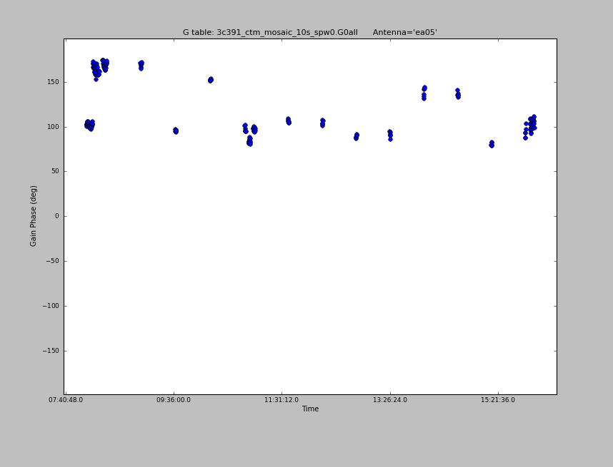
To really see what is going on, we use plotcal to inspect the solutions for a single antenna at a time, iterating through each antenna in sequence, starting with the R polarization:
# In CASA
plotcal(caltable='3c391_ctm_mosaic_10s_spw0.G0all',xaxis='time',yaxis='phase',
        poln='R',iteration='antenna',plotrange=[-1,-1,-180,180])
You use the Next button on the GUI to advance the displayed antenna. In Figure 5 we have stepped through to antenna ea05.
NOTE: Sometimes plotcal will lock a table and/or keep it in the table cache beyond the end of plotting. This can hang up further use of that table, or cause errors if you delete the table outside of CASA and want to re-create it. To deal with that issue, simply close the plotcal GUI using the Quit button when you are done looking at the plot.
Antennas that have been flagged will show a blank plot, as there are no solutions for these antennas. For most antennas, we see a fairly smooth variation with time, so we expect to be able to calibrate our data nicely. However, when you get to ea05, note the phase jumps where it appears to be bouncing between two states. We can plot this antenna separately:
# In CASA
plotcal(caltable='3c391_ctm_mosaic_10s_spw0.G0all',xaxis='time',yaxis='phase',antenna='ea05',
        poln='R',iteration='antenna',plotrange=[-1,-1,-180,180],figfile='plotcal_3c391-G0all-phase-R-ea05.png')
We see the same thing for the L polarization solutions:
# In CASA
plotcal(caltable='3c391_ctm_mosaic_10s_spw0.G0all',
        xaxis='time', yaxis='phase', poln='L',
        iteration='antenna', plotrange=[-1,-1,-180,180])
Antennas other than ea05 look OK.
We will not be able to transfer calibration for antenna ea05 so we will flag it from the data:
# In CASA
flagdata(vis='3c391_ctm_mosaic_10s_spw0.ms',
         flagbackup=T, mode='manual', antenna='ea05')
For the following bandpass solution we need only solve for our bandpass calibrator, and we will do so now after flagging:
# In CASA
gaincal(vis='3c391_ctm_mosaic_10s_spw0.ms', caltable='3c391_ctm_mosaic_10s_spw0.G0',
        field='J1331+3030', refant='ea21', spw='0:27~36', calmode='p', solint='int',
        minsnr=5, gaintable=['3c391_ctm_mosaic_10s_spw0.antpos'])
You can inspect this with plotcal as we did above. For example, plot R for the first block of 3C286 data only:
# In CASA
plotcal(caltable='3c391_ctm_mosaic_10s_spw0.G0',
        xaxis='time',yaxis='phase',poln='R',field='J1331+3030',iteration='antenna',
        plotrange=[-1,-1,-180,180],timerange='08:02:00~08:17:00')
You can do the same for L if you like.
Delay Calibration
The first stage of bandpass calibration involves solving for the antenna-based delays which put a phase ramp versus frequency channel in each spectral window. The K gain type in gaincal solves for the relative delays of each antenna relative to the reference antenna (parameter refant), so be sure you pick one that is there for this entire scan and good. This is not a full global delay, but gives one value per spw per polarization.
# In CASA
gaincal(vis='3c391_ctm_mosaic_10s_spw0.ms',caltable='3c391_ctm_mosaic_10s_spw0.K0',
        field='J1331+3030',refant='ea21',spw='0:5~58',gaintype='K',
        solint='inf',combine='scan',minsnr=5,
        gaintable=['3c391_ctm_mosaic_10s_spw0.antpos',
                   '3c391_ctm_mosaic_10s_spw0.G0'])
- field='J1331+3030' : For the bandpass calibrator
- refant='ea21' : Delays will be relative to this antenna, make sure it is there!
- spw='0:5~58' : Widest possible frequency range in the spw, avoiding edge channels
- gaintype='K' : Compute K solutions, one per antenna per spw per polarization per solution interval
- solint='inf',combine='scan' : Only need one solution averaged over all times and scans
- minsnr=5 : One probably wants to restrict the solutions to be at relatively high signal-to-noise ratios, although this parameter may need to be varied depending upon the source and frequency.
- gaintable=['3c391_ctm_mosaic_10s_spw0.antpos','3c391_ctm_mosaic_10s_spw0.G0'] : Use the antpos and G0 tables.
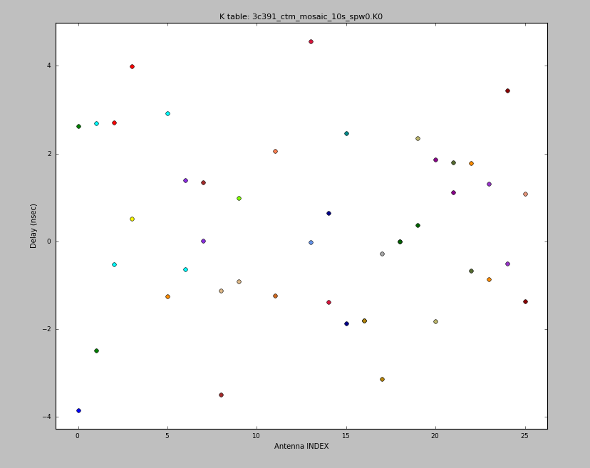
We can plot these solutions (in nanoseconds) as a function of antenna:
# In CASA
plotcal(caltable='3c391_ctm_mosaic_10s_spw0.K0',xaxis='antenna',yaxis='delay',
        figfile='plotcal_3c391-K0-delay.png')
These are within about 4 nanoseconds, as expected for the early JVLA science observations.
Bandpass Calibration
This step solves for the complex bandpass, [math]\displaystyle{ B_i }[/math].
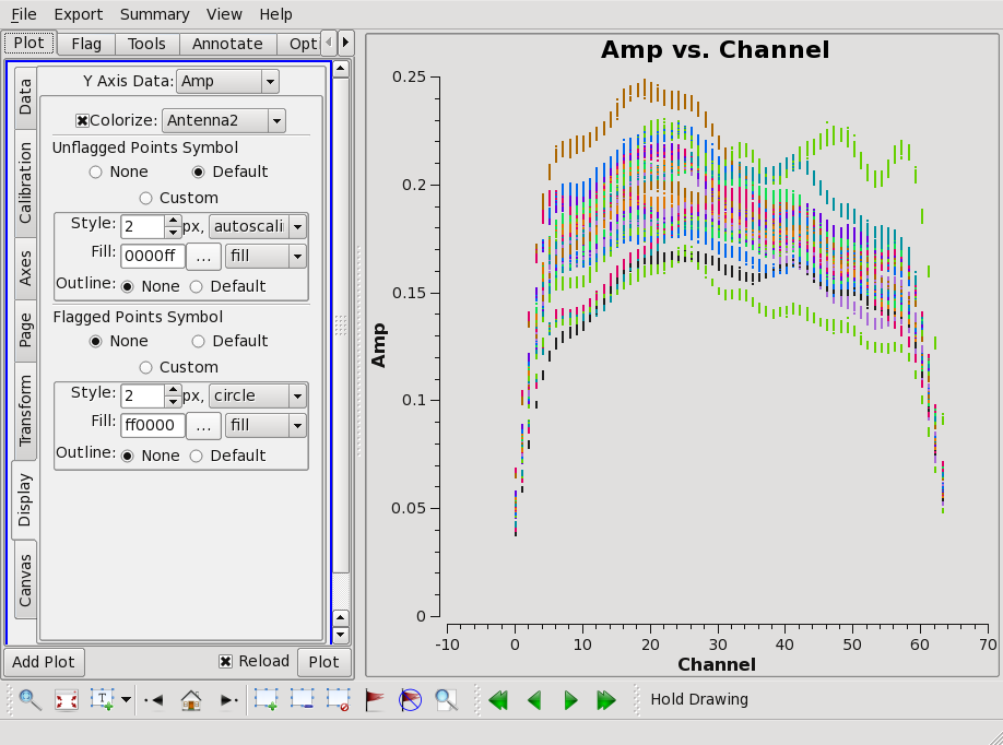
For the VLA, in its old continuum modes, this step could be skipped. With the JVLA, all data are spectral line, even if the science that one is conducting is continuum. Solving for the bandpass won't hurt for continuum data, and, for moderate or high dynamic range image, it is essential. To motivate the need for solving for the bandpass, consider Figure 7. It shows the right circularly polarized data (RR polarization) for the source J1331+3030, which will serve as the bandpass calibrator. The data are color coded by spectral window, and they are averaged over all baselines, as earlier plots from plotms indicated that the visibility data are nearly constant with baseline length. Ideally, the visibility data would be constant as a function of frequency as well. The variations with frequency are a reflection of the (slightly) different antenna bandpasses. (>Exercise for the reader, reproduce Figure 7 using plotms.)
Now form the bandpass, using the phase solutions just derived.
# In CASA
bandpass(vis='3c391_ctm_mosaic_10s_spw0.ms',caltable='3c391_ctm_mosaic_10s_spw0.B0',
         field='J1331+3030',spw='',refant='ea21',solnorm=True,combine='scan',
         solint='inf',bandtype='B',
         gaintable=['3c391_ctm_mosaic_10s_spw0.antpos',
                    '3c391_ctm_mosaic_10s_spw0.G0',
                    '3c391_ctm_mosaic_10s_spw0.K0'])
- caltable='3c391_ctm_mosaic_10s_spw0.B0' : Specify where to store the bandpass corrections.
- solnorm=T : Make sure that the average of the amplitudes of the bandpass corrections are normalized to unity (across the spw)
- solint='inf', combine='scan' : This observation contains multiple scans on the bandpass calibrator, J1331+3030. Because these are continuum observations, it is probably acceptable to combine all the scans and compute one bandpass correction per antenna, which is achieved by the combination of 'solint='inf' and combine='scan' . Had combine=' ' then there would have been a bandpass correction derived per scan, which might be necessary for the highest dynamic range spectral line observations.
- bandtype='B' : The bandpass solution will be derived on a channel-by-channel basis. There is an alternate, somewhat experimental option of parameter bandtype='BPOLY' that will attempt to fit an nth order polynomial to the bandpass.
- gaintable=['3c391_ctm_mosaic_10s_spw0.antpos','3c391_ctm_mosaic_10s_spw0.G0','3c391_ctm_mosaic_10s_spw0.K0'] : Pre-apply antenna positions, phase solutions, and delays.
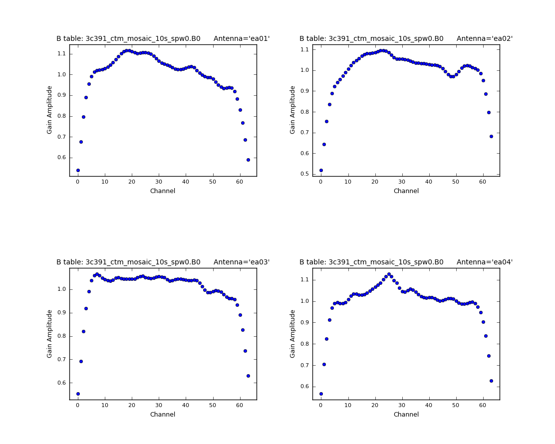
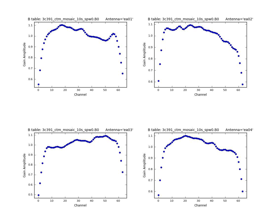
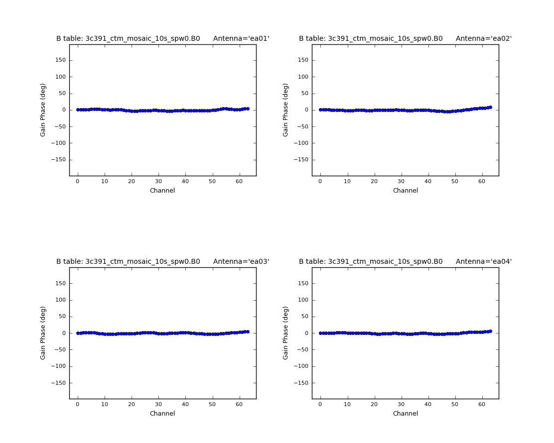
Once again, one can use plotcal to display the bandpass solutions. Note that in the plotcal inputs below, the amplitudes are being displayed as a function of frequency channel and, for compactness, parameter subplot=221 is used to display multiple plots per page; you could have used paramter yaxis='phase' to view the phases as well. Parameter iteration='antenna' is used to step through separate plots for each antenna.
# In CASA
plotcal(caltable= '3c391_ctm_mosaic_10s_spw0.B0',poln='R',
        xaxis='chan',yaxis='amp',field= 'J1331+3030',subplot=221,
        iteration='antenna',figfile='plotcal_3c391-3C286-B0-R-amp.png')
#
plotcal(caltable= '3c391_ctm_mosaic_10s_spw0.B0',poln='L',
        xaxis='chan',yaxis='amp',field= 'J1331+3030',subplot=221,
        iteration='antenna',figfile='plotcal_3c391-3C286-B0-L-amp.png')
#
plotcal(caltable= '3c391_ctm_mosaic_10s_spw0.B0',poln='R',
        xaxis='chan',yaxis='phase',field= 'J1331+3030',subplot=221,
        iteration='antenna',plotrange=[-1,-1,-180,180],
        figfile='plotcal_3c391-3C286-B0-R-phase.png')
#
plotcal(caltable= '3c391_ctm_mosaic_10s_spw0.B0',poln='L',
        xaxis='chan',yaxis='phase',field= 'J1331+3030',subplot=221,
        iteration='antenna',plotrange=[-1,-1,-180,180],
        figfile='plotcal_3c391-3C286-B0-L-phase.png')
As expected, the bandpass phases are relatively flat (see Figures 8A–8D), with the slopes removed by the delay calibration. Residual excursions are on the order of a few degrees.
 |
 |
 |
 |
Gain Calibration
The next step is to derive corrections for the complex antenna gains, [math]\displaystyle{ g_i }[/math] and [math]\displaystyle{ \theta_i }[/math]. As discussed above, the absolute magnitude of the gain amplitudes—[math]\displaystyle{ g_i }[/math]—are determined by reference to a standard flux density calibrator. In order to determine the appropriate complex gains for the target source, and to minimize differences through the atmosphere (neutral and/or ionized) between the lines of sight to the phase calibrator and the target source, you want to observe a so-called phase calibrator that is much closer to the target. If we establish the relative gain amplitudes and phases for different antennas using the phase calibrator, we can later determine the absolute flux density scale by comparing the gain amplitudes, [math]\displaystyle{ g_i }[/math], derived for 3C 286 with those derived for the phase calibrator. This will eventually be done using the task fluxscale. Since there is no such thing as absolute phase, we determine a zero phase by selecting a reference antenna for which the gain phase is defined to be zero.
In principle, one could determine the complex antenna gains for all sources with a single invocation of gaincal; for clarity here, two separate invocations will be used.
In the first step, we derive the appropriate complex gains [math]\displaystyle{ g_i }[/math] and [math]\displaystyle{ \theta_i }[/math] for the flux density calibrator 3C 286.
# In CASA
gaincal(vis='3c391_ctm_mosaic_10s_spw0.ms',caltable='3c391_ctm_mosaic_10s_spw0.G1',
        field='J1331+3030',spw='0:5~58',
        solint='inf',refant='ea21',gaintype='G',calmode='ap',solnorm=F,
        gaintable=['3c391_ctm_mosaic_10s_spw0.antpos',
                   '3c391_ctm_mosaic_10s_spw0.K0',
                   '3c391_ctm_mosaic_10s_spw0.B0'])
- caltable='3c391_ctm_mosaic_10s_spw0.G1' : Produce a new calibration table containing these gain solutions. In order to make the bookkeeping easier, a '1' is appended to the file name to distinguish it from the earlier set of gain solutions, which are effectively being thrown away.
- spw='0:5~58' : From the inspection of the bandpass, one can determine the range of edge channels that are affected by the bandpass filter rolloff. Because the amplitude is dropping rapidly in these channels, one does not want to include them in the solution.
- gaintype='G', calmode='ap', solnorm=F : Solve for the complex antenna gains for 3C 286. The objective is to relate the measured data values to the (assumed known) flux density of 3C 286, thus the solution is both amplitude and phase ('ap') and the solutions should not be normalized to unity amplitude.
- solint='inf' : Produce a solution for each scan. Phase coherence for these observations is good.
- gaintable=['3c391_ctm_mosaic_10s_spw0.antpos','3c391_ctm_mosaic_10s_spw0.K0','3c391_ctm_mosaic_10s_spw0.B0'] : Use the antenna position corrections, delays, and bandpass solutions determined earlier before solving for the gain amplitudes.
In the second step, the appropriate complex gains for a direction on the sky close to the target source will be determined from the phase calibrator J1822-0938. We also determine the complex gains for the polarization calibrator source J0319+4130. These will be solved separately, but in practice could be solved together as there are no gaintables that are time dependent at this point (and thus would risk having cross-source interpolation issues), nor are we doing different solution intervals per source.
# In CASA
gaincal(vis='3c391_ctm_mosaic_10s_spw0.ms',caltable='3c391_ctm_mosaic_10s_spw0.G1',
        field='J1822-0938',
        spw='0:5~58',solint='inf',refant='ea21',gaintype='G',calmode='ap',
        gaintable=['3c391_ctm_mosaic_10s_spw0.antpos',
                   '3c391_ctm_mosaic_10s_spw0.K0',
                   '3c391_ctm_mosaic_10s_spw0.B0'],
        append=True)
#
gaincal(vis='3c391_ctm_mosaic_10s_spw0.ms',caltable='3c391_ctm_mosaic_10s_spw0.G1',
        field='J0319+4130',
        spw='0:5~58',solint='inf',refant='ea21',gaintype='G',calmode='ap',
        gaintable=['3c391_ctm_mosaic_10s_spw0.antpos',
                   '3c391_ctm_mosaic_10s_spw0.K0',
                   '3c391_ctm_mosaic_10s_spw0.B0'],
        append=True)
- caltable='3c391_ctm_mosaic_10s_spw0.G1', append=True : In all previous invocations of gaincal, append has been set to False. Here, the gain solutions from the phase calibrators are going to be appended to the existing set from 3C 286. In following steps, all of these gain solutions will then be used together to derive a set of complex gains that are applied to the science data for the target source.
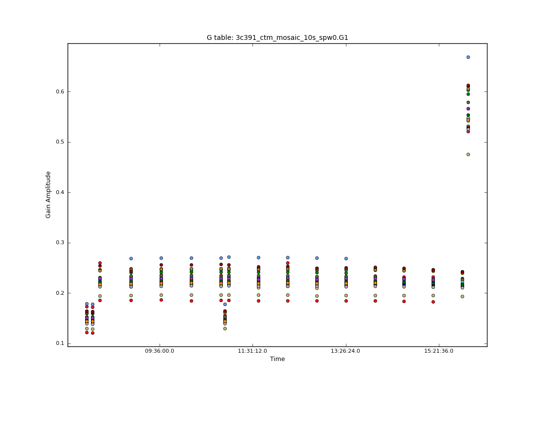
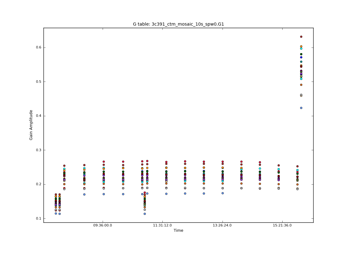
If one checks the gain phase solutions using plotcal, one should see smooth solutions for each antenna as a function of time (see Figures 9A–9D).
# In CASA
plotcal(caltable='3c391_ctm_mosaic_10s_spw0.G1',xaxis='time',yaxis='phase',
        poln='R',plotrange=[-1,-1,-180,180],figfile='plotcal_3c391-G1-phase-R.png')
plotcal(caltable='3c391_ctm_mosaic_10s_spw0.G1',xaxis='time',yaxis='phase',
        poln='L',plotrange=[-1,-1,-180,180],figfile='plotcal_3c391-G1-phase-L.png')
plotcal(caltable='3c391_ctm_mosaic_10s_spw0.G1',xaxis='time',yaxis='amp',
        poln='R',figfile='plotcal_3c391-G1-amp-R.png')
plotcal(caltable='3c391_ctm_mosaic_10s_spw0.G1',xaxis='time',yaxis='amp',
        poln='L',figfile='plotcal_3c391-G1-amp-L.png')
 |
 |
 |
 |
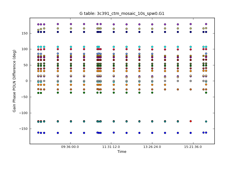
This is also a good time to check that our chosen reference antenna (ea21) has good phase stability (i.e., the phase difference between the right and left polarizations is stable with time). This is a prerequisite for accurate polarization calibration. To do this, we plot the complex polarization ratio:
# In CASA
plotcal(caltable='3c391_ctm_mosaic_10s_spw0.G1', xaxis='time', yaxis='phase',
        poln='/', plotrange=[-1,-1,-180,180], figfile='plotcal_3c391-G1-phase-rat.png')
As can be seen in Figure 10, there is a bit of drift (a few degrees here and there), but no phase jumps. This means that ea21 is, indeed, a good choice for reference antenna.
 |
Polarization Calibration
[If time is running short, skip this step and proceed to Applying the Calibration below.]
Having set the complex gains, we now need to do the polarization calibration. This should be done prior to running fluxscale, since it has to run using the un-rescaled gains in the MODEL_DATA column of the measurement set. Polarization calibration is done in two steps. First, we solve for the instrumental polarization (the frequency-dependent leakage terms, or 'D-terms'), using either an unpolarized source or a source which has sufficiently good parallactic angle coverage. Second, we solve for the polarization position angle using a source with a known polarization position angle (3C 286 is recommended here).
Our initial run of setjy only set the total intensity of our flux calibrator source, 3C 286. This source is known to have a fairly stable fractional polarization (measured to be 11.2% in C-band around the time of the observations), and a polarization position angle of 33 degrees (at most frequencies). For information on polarization calibrators suitable for VLA observations, see the VLA Observing Guide to Polarimetry. The most recently determined values (given in a table at the bottom of the Polarimetry guide page) give 11.3% at 4.5GHz, but below we use the old value of 11.2% for consistency with the rest of the guide.
In order to calibrate the position angle, we need to set the appropriate values for Stokes Q and U. Examining our casapy.log file to find the output of setjy, we find that the total intensity was set to 7.6677 Jy in channel 0 of spw 0, at 4536 MHz according to the listobs output. We therefore use python to find the polarized flux, P, and the values of Stokes Q and U at this reference channel:
# In CASA
i0=7.6677 # Stokes I value for spw 0 ch 0
p0=0.112*i0 # Fractional polarization=11.2%
q0=p0*cos(66*pi/180) # Stokes Q for spw 0 for pang = 33deg (Q+iU phase = 66deg)
u0=p0*sin(66*pi/180) # Stokes U for spw 0 for pang = 33deg (Q+iU phase = 66deg)
Furthermore, since CASA 3.4, we can introduce a spectral index to the flux densities. We do this by noting that our printout from setjy gave 7.53261 Jy in the last channel 127 (at 4663 MHz). Therefore we use python again to compute a spectral index
# In CASA
alpha = log(7.53261/7.6677)/log(4663.0/4536.0)
which gives alpha = -0.64371.
We now set the values of Stokes I, Q and U for 3C 286, using setjy using the abovevalues. First, because we still have the old I-only model in the header, we will delete this:
# In CASA
delmod('3c391_ctm_mosaic_10s_spw0.ms')
NOTE: In CASA 4.0 if you do not do this delmod both the old and new models will be in the header and will be used, doubling the fluxes and confusing other tasks. In future releases we will have the second setjy properly replace the old model.
Now we generate the polarization model:
# In CASA
setjy(vis='3c391_ctm_mosaic_10s_spw0.ms',field='J1331+3030',standard='manual',
      spw='0',fluxdensity=[i0,q0,u0,0],spix=[alpha,0],reffreq='4536.0MHz',
      scalebychan=True,usescratch=False)
- standard='manual' : The user is going to supply the flux densities rather than giving a model
- fluxdensity=[i0,q0,u0,0] : use the IQUV values for channel 0 calculated above
- spix=alpha : Set the spectral index using the formula above (this will also apply to QU)
- reffreq='4536.0MHz' : The frequency of channel 0 from listobs
- scalebychan=True : let it compute a value per channel
- usescratch=False : DO NOT create/use the MODEL_DATA column explicitly
The Stokes V flux value has been set to zero, corresponding to no circular polarization.
Note: In CASA 4.2 the setjy task parameters have changed, in particular the use of standard='manual' to specify flux densities. CASA 4.3 added the polindex, polangle and rotmeas capability, although as of 4.3.1 it will not work correctly for all values of polangle and thus is still experimental. Beware when following this guide with earlier versions.
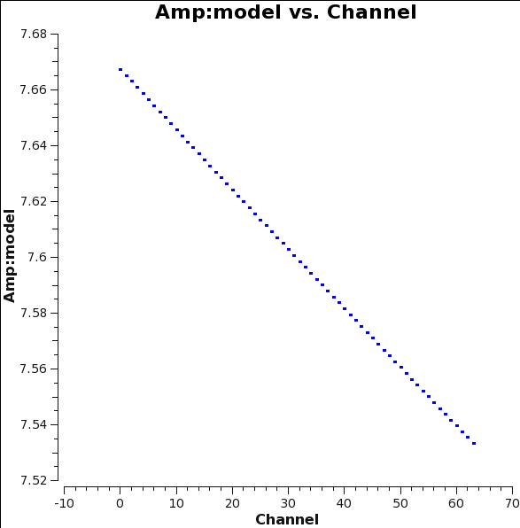
We can see the results in the model column in plotms
# In CASA
plotms(vis='3c391_ctm_mosaic_10s_spw0.ms',field='0',correlation='RR',
       timerange='08:02:00~08:17:00',antenna='ea01&ea02',
       xaxis='channel',yaxis='amp',ydatacolumn='model',
       plotfile='plotms_3c391-model-amp-RR.png',overwrite=True)
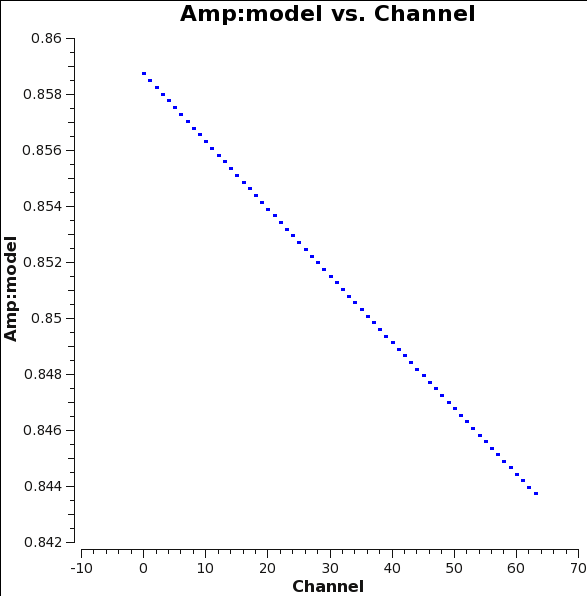
showing our model source spectrum. We can see this translates to the spectrum in QU
# In CASA
plotms(vis='3c391_ctm_mosaic_10s_spw0.ms',field='0',correlation='RL',
       timerange='08:02:00~08:17:00',antenna='ea01&ea02',
       xaxis='channel',yaxis='amp',ydatacolumn='model',
       plotfile='plotms_3c391-model-amp-RL.png',overwrite=True)
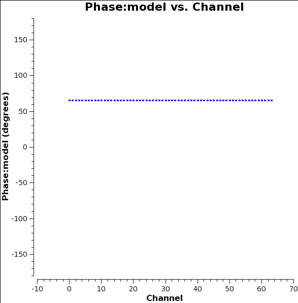
Finally, our R-L phase difference is constant at 66 degrees (twice the polarization angle) as desired:
# In CASA
plotms(vis='3c391_ctm_mosaic_10s_spw0.ms',field='0',correlation='RL',
       timerange='08:02:00~08:17:00',antenna='ea01&ea02',
       xaxis='channel',yaxis='phase',ydatacolumn='model',
       plotrange=[-1,-1,-180,180],plotfile='plotms_3c391-model-phase-RL.png',
       overwrite=True)
 |
 |
 |
Solving for the Cross-Hand delays
Just as we did for the parallel-hand (RR,LL) delays before bandpass calibration, we solve for the cross-hand (RL,LR) delays due to the residual delay difference between the R and L on the reference antenna (ea21) used for the original delay calibration. In our case we simply use 3C286 which has a strong polarized signal in the RL,LR correlations.
# In CASA
gaincal(vis='3c391_ctm_mosaic_10s_spw0.ms', caltable='3c391_ctm_mosaic_10s_spw0.Kcross',
        field='J1331+3030', spw='0:5~58',
        gaintype='KCROSS', solint='inf', combine='scan', refant='ea21',
        gaintable=['3c391_ctm_mosaic_10s_spw0.antpos',
                   '3c391_ctm_mosaic_10s_spw0.K0',
                   '3c391_ctm_mosaic_10s_spw0.B0',
                   '3c391_ctm_mosaic_10s_spw0.G1'],
        gainfield=['','','','J1331+3030'],
        interp=['linear','nearest','nearest','linear'], parang=T)
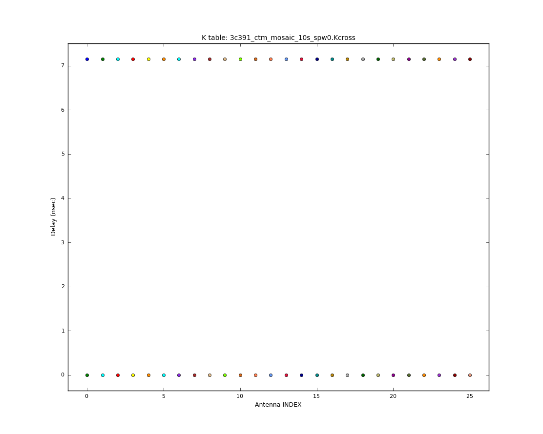
We can plot these:
# In CASA
plotcal(caltable='3c391_ctm_mosaic_10s_spw0.Kcross',xaxis='antenna',yaxis='delay',
        figfile='plotcal_3c391-Kcross-delay.png')
As expected there is a single value for R versus L (with L delay set to zero) across all antennas. The solution is reported in the logger, and is 7.149 ns.
Note that if we did not solve for this delay, it would be absorbed into the phases per channel of the following Df and Xf solutions. This would not cause us problems, as we are not solving for the Q+iU polarization of our D-term calibrator (we are using unpolarized 3C84 for that) but if we were (e.g. using our gain calibrator J1822-0938 with poltype='Df+QU') then this step would be essential.
Solving for the Leakage Terms
The task polcal is used for polarization calibration. In this data set, we observed the unpolarized calibrator J0319+4130 (a.k.a. 3C 84) in order to solve for the instrumental polarization. polcal uses the Stokes I, Q, and U values in the MODEL_DATA column (Q and U being zero for our unpolarized calibrator) to derive the leakage solutions. The function call is
# In CASA
polcal(vis='3c391_ctm_mosaic_10s_spw0.ms',caltable='3c391_ctm_mosaic_10s_spw0.D1',
       field='J0319+4130',spw='0:5~58',
       refant='ea21',poltype='Df',solint='inf',combine='scan',
       gaintable=['3c391_ctm_mosaic_10s_spw0.antpos',
                  '3c391_ctm_mosaic_10s_spw0.K0',
                  '3c391_ctm_mosaic_10s_spw0.B0',
                  '3c391_ctm_mosaic_10s_spw0.G1',
                  '3c391_ctm_mosaic_10s_spw0.Kcross'],
       gainfield=['','','','J0319+4130',''],
       interp=['linear','nearest','nearest','linear','nearest'])
- caltable='3c391_ctm_mosaic_10s_spw0.D1' : polcal will create a new calibration table containing the leakage solutions, which we specify with the caltable argument.
- field='J0319+4130' : The unpolarized source J0319+4130 (a.k.a. 3C 84) is used to solve for the leakage terms.
- spw='0:5~58' : In this example, the edge channels are not used in finding the solution. Because the bandpass is one of the calibration tables being applied (in gaintable), this restriction is not necessary. However, if one restricts the spectral window here, it must also be restricted in the remainder of the calibration steps, particularly applycal, otherwise the final data set will contain frequency channels for which the leakage terms have not been calibrated.
- poltype='Df' : We will solve for the leakages (D) on a per-channel basis (f) assuming zero source polarization.
- solint='inf' : One solution over the entire run (the default)
- combine='scan' : Combine all scans together (the default)
- gaintable : All of the previous corrections---antenna positions, K-delay, bandpass, Kcross-delay, and complex gain---are to be applied
- gainfield : The gain caltable that is being applied on the fly, 3c391_ctm_mosaic_10s_spw0.G1, contains the solutions for multiple sources. Only the solutions from J0319+4130 should be applied to itself in the process of finding the polarization leakage terms.
- interp : The interpolation to be used for each gaintable.
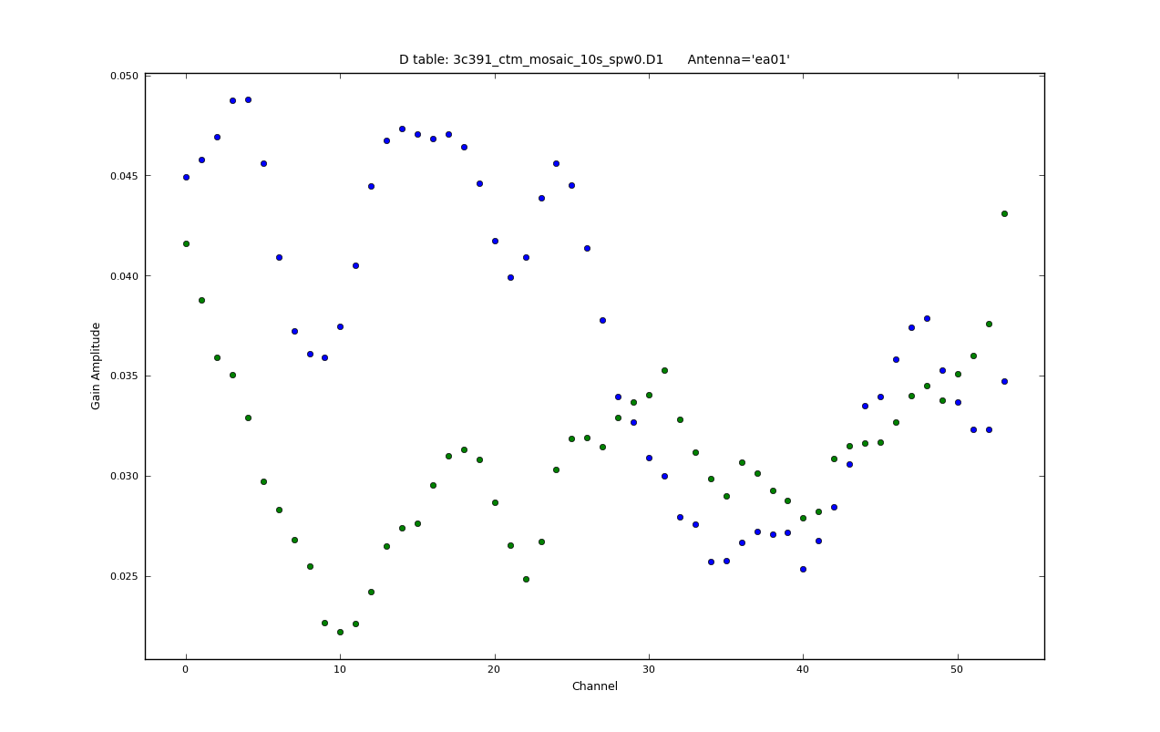
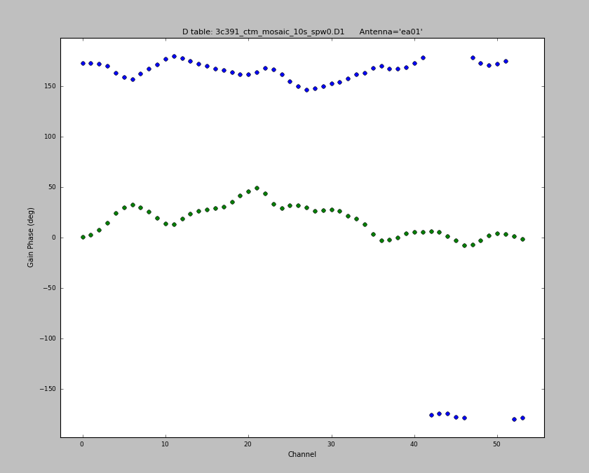
After polcal has finished running, you are strongly advised to examine the solutions with plotcal, to ensure that everything looks good.
# In CASA
plotcal(caltable='3c391_ctm_mosaic_10s_spw0.D1',xaxis='chan',yaxis='amp',
        spw='',field='',iteration='antenna')
#
plotcal(caltable='3c391_ctm_mosaic_10s_spw0.D1',xaxis='chan',yaxis='phase',
        spw='',field='',iteration='antenna',plotrange=[-1,-1,-180,180])
This will produce plots similar to those shown at right (you might get slightly different values). As ever, you can cycle through the antennas by clicking the Next button. You should see leakages of between 5 and 15% in most cases. We can also display these in a single plot versus antenna index:
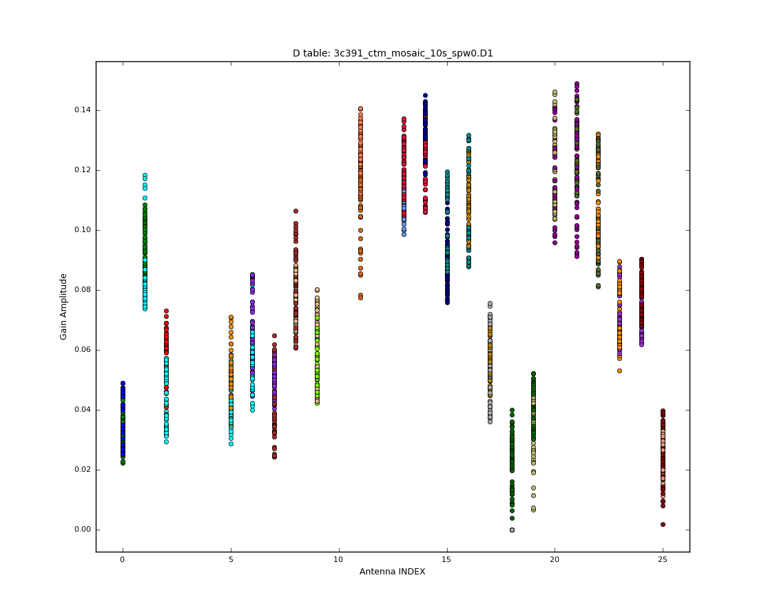
# In CASA
plotcal(caltable='3c391_ctm_mosaic_10s_spw0.D1',xaxis='antenna',yaxis='amp',
        figfile='plotcal_3c391-D1.png')
Note that there are no solutions for antenna ea04 - a bit of sleuthing will turn up that ea04 was missing for the scans on 3C84.
If we want to rescue ea04 (which otherwise seems ok) then we turn to our gain calibrator. If we plot data for field 1 versus ParAngle in plotms then we see that it has sufficient range (>60 deg) in parallactic angle so should be useable as a calibrator with unknown polarization. We can make a new set of solutions:
# In CASA
polcal(vis='3c391_ctm_mosaic_10s_spw0.ms',caltable='3c391_ctm_mosaic_10s_spw0.D2',
       field='J1822-0938',spw='0:5~58',
       refant='ea21',poltype='Df+QU',solint='inf',combine='scan',
       gaintable=['3c391_ctm_mosaic_10s_spw0.antpos',
                  '3c391_ctm_mosaic_10s_spw0.K0',
                  '3c391_ctm_mosaic_10s_spw0.B0',
                  '3c391_ctm_mosaic_10s_spw0.G1',
                  '3c391_ctm_mosaic_10s_spw0.Kcross'],
       gainfield=['','','','J1822-0938',''],
       interp=['linear','nearest','nearest','linear','nearest'])
- field='J1822-0938' : Our gain calibrator observed throughout the schedule block
- poltype='Df+QU' : Solve for the leakages using a calibrator with unknown polarization but with good parallactic angle coverage, and simultaneously for the source polarization (averaged over frequency)
- gainfield : For 3c391_ctm_mosaic_10s_spw0.G1 use only the solutions from J1822-0938 itself.
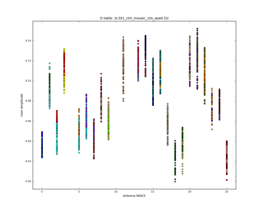
We now plot this as we did before:
# In CASA
plotcal(caltable='3c391_ctm_mosaic_10s_spw0.D2',xaxis='antenna',yaxis='amp',
        figfile='plotcal_3c391-D2.png')
Comparison of this plot with that for the D1 caltable shows that we get nearly identical results, but now ea04 (index 3) is present! That should give us some confidence in our leakage calibration as well.
Solving for the R-L polarization angle
Having calibrated the instrumental polarization, the total polarization is now correct, but the R-L phase still needs to calibrated in order to obtain an accurate polarization position angle. We use the same task, polcal, but this time set poltype='Xf, which specifies a frequency-dependent (f) position angle (X) calibration, using the source J1331+3030 (a.k.a. 3C 286), whose position angle is known, having set this earlier using setjy. Note that we must correct for the leakages before determining the R-L phase, which we do by adding the calibration table made in the previous step (3c391_ctm_mosaic_10s_spw0.D2) to the gain tables that are applied on-the-fly. Note that we are using the second D table we made as it included ea04.
# In CASA
polcal(vis='3c391_ctm_mosaic_10s_spw0.ms',caltable='3c391_ctm_mosaic_10s_spw0.X1',
       field='J1331+3030',combine='scan',
       poltype='Xf',solint='inf',
       gaintable=['3c391_ctm_mosaic_10s_spw0.antpos',
                  '3c391_ctm_mosaic_10s_spw0.K0',
                  '3c391_ctm_mosaic_10s_spw0.B0',
                  '3c391_ctm_mosaic_10s_spw0.G1',
                  '3c391_ctm_mosaic_10s_spw0.Kcross',
                  '3c391_ctm_mosaic_10s_spw0.D2'],
       gainfield=['','','','J1331+3030','',''],
       interp=['linear','nearest','nearest','linear','nearest','nearest'])
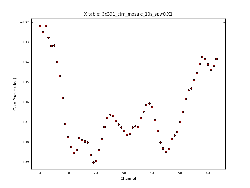
Again, it is strongly suggested that you check the calibration worked properly, by plotting up the newly-generated calibration table using plotcal. The results are shown at right.
# In CASA
plotcal(caltable='3c391_ctm_mosaic_10s_spw0.X1',xaxis='chan',yaxis='phase',
        figfile='plotcal_3c391-X1.png')
Because the Xf term captures the residual R-L phase on the reference antenna over the array, there is one value for all antennas. Also, as we took out the RL delays using the Kcross solution, these Xf variations only span about 6 degress across the spectral window.
At this point, you have all the necessary polarization calibration tables.
Scaling the Amplitude Gains
While we know the flux density of our primary calibrator (in our case, J1331+3030[math]\displaystyle{ \equiv }[/math]3C 286), the model assumed for the secondary calibrator (here, J1822-0938) was a point source of 1 Jy located at the phase center. While the secondary calibrator was chosen to be a point source (at least, over some limited range of uv-distance; see the VLA calibrator manual for any u-v restrictions on your calibrator of choice at the observing frequency), its absolute flux density is unknown. Being pointlike, secondary calibrators typically vary on timescales of months to years, in some cases by up to 50--100%.
We use the primary calibrator (the 'flux calibrator') to determine the system response to a source of known flux density, and assume that the mean gain amplitudes for the primary calibrator are the same as those for the secondary calibrator. This then allows us to find the true flux density of the secondary calibrator. To do this, we use the task fluxscale, which produces a new calibration table containing properly-scaled amplitude gains for the secondary calibrator.
# In CASA
myscale = fluxscale(vis='3c391_ctm_mosaic_10s_spw0.ms',
                    caltable='3c391_ctm_mosaic_10s_spw0.G1',
                    fluxtable='3c391_ctm_mosaic_10s_spw0.fluxscale1',
                    reference=['J1331+3030'],
                    transfer=['J1822-0938,J0319+4130'],
                    incremental=False)
- myscale = fluxscale() : fluxscale returns a dictionary of results, which we capture in the variable myscale
- caltable='3c391_ctm_mosaic_10s_spw0.G1' : We provide fluxscale with the calibration table containing the amplitude gain solutions derived earlier.
- fluxtable='3c391_ctm_mosaic_10s_spw0.fluxscale1' : We specify the name of the new output table to be written, which will contain the properly-scaled amplitude gains.
- reference='J1331+3030' : We specify the source with the known flux density.
- transfer=['J1822-0938,J0319+4130'] : We specify the sources whose amplitude gains are to be rescaled.
- incremental=False : Make a new output fluxtable replacing caltable with rescaled transfer gains. If True then the new table would be used in addition to caltable in subsequent applications.
fluxscale will print to the CASA logger the derived flux densities of all calibrator sources specified with the transfer argument. These are also captured in the return variable from the task. You should examine the output to ensure that it looks sensible. If one's data set has more than 1 spectral window, depending upon where they are spaced and the spectrum of the source, it is quite possible to find (quite) different flux densities and spectral indexes for the secondary calibrators. Example output would be
CASA <99>: myscale['1']
  Out[99]:
{'0': {'fluxd': array([ 2.29522371,  0.        ,  0.        ,  0.        ]),
       'fluxdErr': array([ 0.00632494,  0.        ,  0.        ,  0.        ]),
       'numSol': array([ 46.,   0.,   0.,   0.])},
 'fieldName': 'J1822-0938',
 'fitFluxd': 0.0,
 'fitFluxdErr': 0.0,
 'fitRefFreq': 0.0,
 'spidx': array([ 0.,  0.,  0.]),
 'spidxerr': array([ 0.,  0.,  0.])}


CASA <100>: myscale['9']
  Out[100]:
{'0': {'fluxd': array([ 13.66191225,   0.        ,   0.        ,   0.        ]),
       'fluxdErr': array([ 0.03827984,  0.        ,  0.        ,  0.        ]),
       'numSol': array([ 44.,   0.,   0.,   0.])},
 'fieldName': 'J0319+4130',
 'fitFluxd': 0.0,
 'fitFluxdErr': 0.0,
 'fitRefFreq': 0.0,
 'spidx': array([ 0.,  0.,  0.]),
 'spidxerr': array([ 0.,  0.,  0.])}
or in the logger
...
Found reference field(s): J1331+3030
 Found transfer field(s):  J1822-0938 J0319+4130
 Flux density for J1822-0938 in SpW=0 (freq=4.599e+09 Hz) is: 2.29522 +/- 0.00632494 (SNR = 362.885, N = 46)
 Flux density for J0319+4130 in SpW=0 (freq=4.599e+09 Hz) is: 13.6619 +/- 0.0382798 (SNR = 356.896, N = 44)
Storing result in 3c391_ctm_mosaic_10s_spw0.fluxscale1
...
Again, the VLA Calibrator Manual may be used to check whether the derived flux densities look sensible. Wildly different flux densities or flux densities with very high error bars should be treated with suspicion; in such cases you will have to figure out whether something has gone wrong.
We plot the rescaled amplitudes from this table:
# In CASA
plotcal(caltable='3c391_ctm_mosaic_10s_spw0.fluxscale1',xaxis='time',yaxis='amp',
        poln='R',figfile='plotcal_3c391-fluxscale1-amp-R.png')
plotcal(caltable='3c391_ctm_mosaic_10s_spw0.fluxscale1',xaxis='time',yaxis='amp',
        poln='L',figfile='plotcal_3c391-fluxscale1-amp-L.png')
You can see (in the plots shown below) that the amplitude gain factors are now similar across sources, compared to the raw factors in the G1 table.
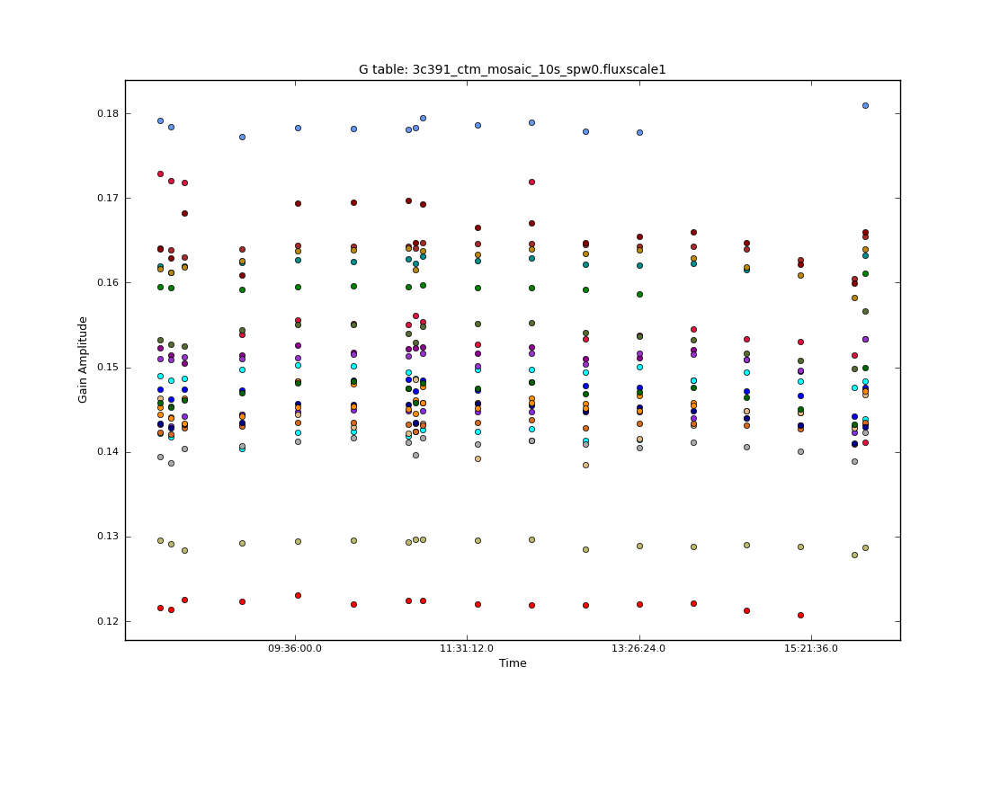 |
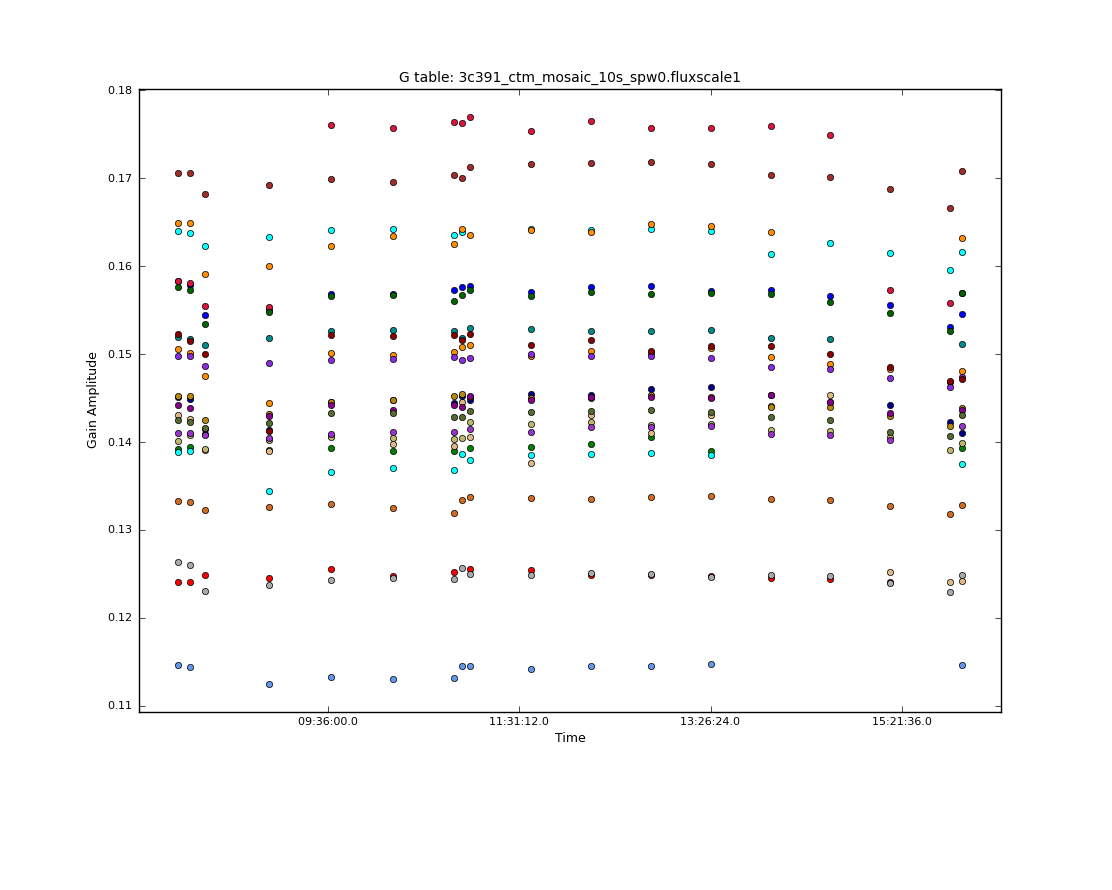 |
Applying the Calibration
Now that we have derived all the calibration solutions, we need to apply them to the actual data, using the task applycal. The measurement set DATA column contains the original data. To apply the calibration we have so painstakingly derived, we specify the appropriate calibration tables, which are then applied to the DATA column, with the results being written in the CORRECTED_DATA column. If the dataset does not already have a CORRECTED_DATA scratch column, then one will be created in the first applycal run.
First, we apply the calibration to each individual calibrator, using the gain solutions derived on that calibrator alone to compute the CORRECTED_DATA. To do this, we iterate over the different calibrators, in each case specifying the source to be calibrated (using the field parameter). The relevant function calls are given below, although as explained presently, the calls to applycal will differ slightly if you skipped the Polarization Calibration steps above.
# In CASA
applycal(vis='3c391_ctm_mosaic_10s_spw0.ms',
         field='J1331+3030',
         gaintable=['3c391_ctm_mosaic_10s_spw0.antpos',
                    '3c391_ctm_mosaic_10s_spw0.fluxscale1',
                    '3c391_ctm_mosaic_10s_spw0.K0',
                    '3c391_ctm_mosaic_10s_spw0.B0',
                    '3c391_ctm_mosaic_10s_spw0.Kcross',
                    '3c391_ctm_mosaic_10s_spw0.D2',
                    '3c391_ctm_mosaic_10s_spw0.X1'],
         gainfield=['','J1331+3030','','','','',''],
         interp=['','nearest','','','','',''],
         calwt=[False],
         parang=True)
#
applycal(vis='3c391_ctm_mosaic_10s_spw0.ms',
         field='J0319+4130',
         gaintable=['3c391_ctm_mosaic_10s_spw0.antpos',
                    '3c391_ctm_mosaic_10s_spw0.fluxscale1',
                    '3c391_ctm_mosaic_10s_spw0.K0',
                    '3c391_ctm_mosaic_10s_spw0.B0',
                    '3c391_ctm_mosaic_10s_spw0.Kcross',
                    '3c391_ctm_mosaic_10s_spw0.D2',
                    '3c391_ctm_mosaic_10s_spw0.X1'],
         gainfield=['','J0319+4130','','','','',''],
         interp=['','nearest','','','','',''],
         calwt=[False],
         parang=True)
#
applycal(vis='3c391_ctm_mosaic_10s_spw0.ms',
         field='J1822-0938',
         gaintable=['3c391_ctm_mosaic_10s_spw0.antpos',
                    '3c391_ctm_mosaic_10s_spw0.fluxscale1',
                    '3c391_ctm_mosaic_10s_spw0.K0',
                    '3c391_ctm_mosaic_10s_spw0.B0',
                    '3c391_ctm_mosaic_10s_spw0.Kcross',
                    '3c391_ctm_mosaic_10s_spw0.D2',
                    '3c391_ctm_mosaic_10s_spw0.X1'],
         gainfield=['','J1822-0938','','','','',''],
         interp=['','nearest','','','','',''],
         calwt=[False],
         parang=True)
- gaintable : We provide a Python list of the calibration tables to be applied. This list must contain the antenna position corrections (in .antpos), the properly-scaled gain calibration for the amplitudes and phases (in .fluxscale1) which were just made using fluxscale, the parallel-hand delays (in .K0), the bandpass solutions (in .B0), the cross-hand delays (in .Kcross), the leakage calibration (in .D2 derived by our second solution), and the R-L phase corrections (in .X1).
- gainfield, interp : To ensure that we use the correct gain amplitudes and phases for a given calibrator (those derived on that same calibrator), then for each calibrator source, we need to specify the particular subset of gain solutions to be applied. This requires use of the gainfield and interp arguments; these are both Python lists, and for the list item corresponding to the calibration table made by fluxscale, we set gainfield to the field name corresponding to that calibrator, and the desired interpolation type (interp) to nearest.
- calwt=[False] : At the time of writing, we are not yet using system calibration data to compute real (1/Jy2) weights, thus trying to calibrate them can produce nonsensical results. In particular, experience has shown that calibrating the weights will lead to problems especially in the self-calibration steps. You can specify calwt on a per-table basis, here is set all to False.
- parang : Since we have performed polarization calibration, we must set parang=True, or we will discard all that hard work we did earlier. However, if you skipped the Polarization_Calibration steps in the section above, the .Kcross, .D2 and .X1 will not exist. In this case, you should leave out these tables from the gaintable list, and the corresponding sets of elements in the gainfield list each time you run applycal above. You should also set parang=False.
Finally, we apply the calibration to the target fields in the mosaic, linearly interpolating the gain solutions from the secondary calibrator, J1822-0938. In this case however, we want to apply the amplitude and phase gains derived from the secondary calibrator, J1822-0938, since that is close to the target source on the sky, and we assume that the gains applicable to the target source are very similar to those derived in the direction of the secondary calibrator. Of course, this is not strictly true, since the gains on J1822-0938 were derived at a different time and in a different position on the sky from the target. However, assuming that the calibrator was sufficiently close to the target, and the weather was sufficiently well-behaved, then this is a reasonable approximation, and should get us a sufficiently good calibration that we can later use self-calibration to correct for the small inaccuracies thus introduced.
The procedure for applying the calibration to the target source is very similar to what we just did for the calibrator sources.
# In CASA
applycal(vis='3c391_ctm_mosaic_10s_spw0.ms',
         field='2~8',
         gaintable=['3c391_ctm_mosaic_10s_spw0.antpos',
                    '3c391_ctm_mosaic_10s_spw0.fluxscale1',
                    '3c391_ctm_mosaic_10s_spw0.K0',
                    '3c391_ctm_mosaic_10s_spw0.B0',
                    '3c391_ctm_mosaic_10s_spw0.Kcross',
                    '3c391_ctm_mosaic_10s_spw0.D2',
                    '3c391_ctm_mosaic_10s_spw0.X1'],
         gainfield=['','J1822-0938','','','','',''],
         interp=['','linear','','','','',''],
         calwt=[False],
         parang=True)
- field : We can calibrate all seven target fields at once by setting field='2~8' .
- gainfield : In this case, we wish to use the gains derived on the secondary calibrator, for the reasons explained in the previous paragraph.
- interp : This time, we linearly interpolate between adjacent calibrator scans, to compute the appropriate gains for the intervening observations of the target.
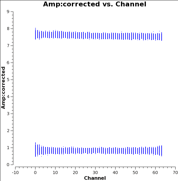 |
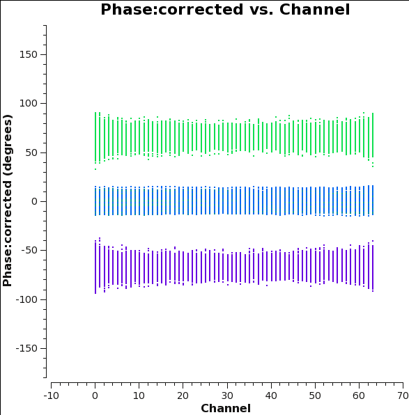 |
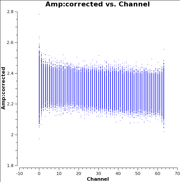 |
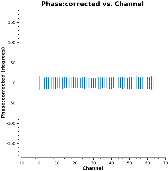 |
We should now have fully-calibrated visibilities in the CORRECTED_DATA column of the measurement set, and it is worthwhile pausing to inspect them, to ensure that the calibration did what we expected it to. We make some standard plots (see above):
# In CASA
plotms(vis='3c391_ctm_mosaic_10s_spw0.ms',field='0',correlation='',
       timerange='08:02:00~08:17:00',antenna='',avgtime='60s',
       xaxis='channel',yaxis='amp',ydatacolumn='corrected',
       plotfile='plotms_3c391-fld0-corrected-amp.png')
#
plotms(vis='3c391_ctm_mosaic_10s_spw0.ms',field='0',correlation='',
       timerange='08:02:00~08:17:00',antenna='',avgtime='60s',
       xaxis='channel',yaxis='phase',ydatacolumn='corrected',
       plotrange=[-1,-1,-180,180],coloraxis='corr',
       plotfile='plotms_3c391-fld0-corrected-phase.png')
#
plotms(vis='3c391_ctm_mosaic_10s_spw0.ms',field='1',correlation='RR,LL',
       timerange='',antenna='',avgtime='60s',
       xaxis='channel',yaxis='amp',ydatacolumn='corrected',
       plotfile='plotms_3c391-fld1-corrected-amp.png')
#
plotms(vis='3c391_ctm_mosaic_10s_spw0.ms',field='1',correlation='RR,LL',
       timerange='',antenna='',avgtime='60s',
       xaxis='channel',yaxis='phase',ydatacolumn='corrected',
       plotrange=[-1,-1,-180,180],coloraxis='corr',
       plotfile='plotms_3c391-fld1-corrected-phase.png')
For 3C286 (leftmost plots) we see the polarized signal in the cross-hands. There is no sign of bad data remaining.
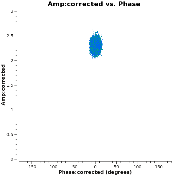
Another nice display is to use plotms to plot the amplitude and phase of the CORRECTED_DATA column against one another, for one of the parallel-hand correlations (RR or LL; the signal in the cross-hands, RL and LR is much smaller, and will be noiselike for an unpolarized calibrator). This should then show a nice ball of visibilities centered at zero phase (with some scatter) and the amplitude found for that source in fluxscale. An example is shown at right.
# In CASA
plotms(vis='3c391_ctm_mosaic_10s_spw0.ms',field='1',correlation='RR,LL',
       timerange='',antenna='',avgtime='60s',
       xaxis='phase',xdatacolumn='corrected',yaxis='amp',ydatacolumn='corrected',
       plotrange=[-180,180,0,3],coloraxis='corr',
       plotfile='plotms_3c391-fld1-corrected-ampvsphase.png')
Inspecting the data at this stage may well show up previously-unnoticed bad data. Plotting up the corrected amplitude against UV distance, or against time is a good way to find such issues. If you find bad data, you can remove them via interactive flagging in plotms, or via manual flagging in flagdata once you have identified the offending antennas/baselines/channels/times. When you are happy that all data (particularly on your target source) look good, you may proceed.
Now that the calibration has been applied to the target data, we can split off the science targets, creating a new, calibrated measurement set containing all the target fields.
# In CASA
split(vis='3c391_ctm_mosaic_10s_spw0.ms',outputvis='3c391_ctm_mosaic_spw0.ms',
      datacolumn='corrected',field='2~8')
- outputvis : We give the name of the new measurement set to be written, which will contain the calibrated data on the science targets.
- datacolumn : We use the CORRECTED_DATA column, containing the calibrated data which we just wrote using applycal.
- field : We wish to put all the mosaic pointings into a single measurement set, for imaging and joint deconvolution.
Initial Imaging
Now that we have split off the target data into a separate measurement set with all the calibration applied, it's time to make an image. Recall from the lectures that the visibility data and the sky brightness distribution (a.k.a. image) are Fourier transform pairs
[math]\displaystyle{ I(l,m) = \int V(u,v) e^{[2\pi i(ul + vm)]} dudv }[/math]
The [math]\displaystyle{ u }[/math] and [math]\displaystyle{ v }[/math] coordinates are the baselines, measured in units of the observing wavelength while the [math]\displaystyle{ l }[/math] and [math]\displaystyle{ m }[/math] coordinates are the direction cosines on the sky. For generality, the sky coordinates are written in terms of direction cosines, but for most EVLA (and ALMA) observations they can be related simply to the right ascension ([math]\displaystyle{ l }[/math]) and declination ([math]\displaystyle{ m }[/math]). Also recall from the lectures that this equation is valid only if the [math]\displaystyle{ w }[/math] coordinate of the baselines can be neglected. This assumption is almost always true at high frequencies and smaller EVLA configurations (such as the 4.6 GHz, D-configuration observations here); the [math]\displaystyle{ w }[/math] coordinate cannot be neglected at lower frequencies and larger configurations (e.g., 0.33 GHz, A-configuration observations). This expression also neglects other factors, such as the shape of the primary beam. For more information on imaging, see Synthesis Imaging within the CASA Reference Manual.
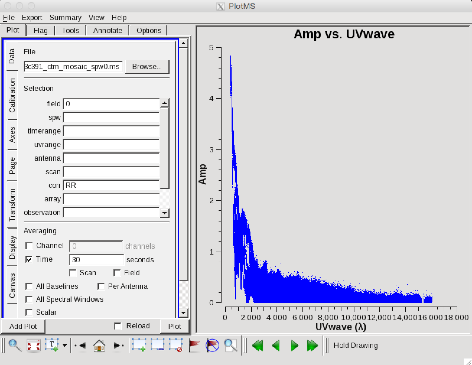
CASA has a single task, clean which both Fourier transforms the data and deconvolves the resulting image. For the purposes of this tutorial Part 1, we will make a simple mosaic clean image in Stokes I only. In Part 2 we will proceed to make multiscale mosaic images in IQUV and to analyze them.
Setting the appropriate pixel size for imaging depends upon basic optics aspects of interferometry. Using plotms to look at the newly-calibrated, target-only data set,
# In CASA
plotms(vis='3c391_ctm_mosaic_spw0.ms',xaxis='uvwave',yaxis='amp',
       ydatacolumn='data', field='0',avgtime='30s',correlation='RR',
       plotfile='plotms_3c391-mosaic0-uvwave.png',overwrite=True)
one should obtain a plot similar to the one shown at the right with the (calibrated) visibility amplitude as a function of [math]\displaystyle{ u }[/math]-[math]\displaystyle{ v }[/math] distance. The maximum baseline is about 16,000 wavelengths, i.e., an angular scale of 12 arcseconds ([math]\displaystyle{ \lambda/D=1/16000 }[/math]). The most effective CLEANing occurs with 3--5 pixels across the synthesized beam. For example, a cell size of 2.5 arcseconds will give just under 5 pixels per beam.
The supernova remnant itself is known to have a diameter of order 9 arcminutes, corresponding to about 216 pixels for the chosen cell size. The mosaic was set up with 7 fields, 1 centered on the remnant and 6 flanking fields; the spacing of the fields was chosen based on the size of the (antenna) primary beam. For the choice of ftmachine='mosaic' (our main mosaicing algorithm), you do not have to fit the mosaic inside the inner quarter of the total image in order to prevent image artifacts arising from aliasing, we just want to have a bit of padding around the outside. Although CASA has the feature that its Fourier transform engine (FFTW) does not require a strict power of 2 for the number of linear pixels in a given image axis, it is somewhat more efficient if the number of pixels on a side is a composite number divisible by any pair of 2 and 3 and/or 5. Because clean internally applies a padding of 1.2 (=3x2/5) choose 480, which is 25 x 3 x 5 (so 480 x 1.2 = 576 = 26 x 32). We therefore set imsize=[480,480] and our mosaic fits comfortably inside the image.
To make this simple clean image interactively:
# In CASA
clean(vis='3c391_ctm_mosaic_spw0.ms',
      imagename='3c391_ctm_spw0_noms_I',
      field='',spw='',
      mode='mfs',
      niter=5000,
      gain=0.1, threshold='1.0mJy',
      psfmode='clark',
      imagermode='mosaic', ftmachine='mosaic',
      multiscale=[0],
      interactive=True,
      imsize=[480,480], cell=['2.5arcsec','2.5arcsec'],
      stokes='I',
      weighting='briggs',robust=0.5,
      usescratch=False)
clean is a powerful task, with many inputs, and a certain amount of experimentation may be (likely is) required.
- vis='3c391_ctm_mosaic_spw0.ms' : this split MS contains our 7-pt mosaic fields, now indexed as 0-6. Field 0 is the central field of the mosaic (you can use listobs to verify this).
- imagename='3c391_ctm_spw0_noms_I' : our output images will all start with this, e.g. 3c391_ctm_spw0_noms_I.image
- mode='mfs' : Use multi-frequency synthesis imaging. The fractional bandwidth of these data is non-zero (128 MHz at a central frequency of 4.6 GHz). Recall that the [math]\displaystyle{ u }[/math] and [math]\displaystyle{ v }[/math] coordinates are defined as the baseline coordinates, measured in wavelengths. Thus, slight changes in the frequency from channel to channel result in slight changes in [math]\displaystyle{ u }[/math] and [math]\displaystyle{ v }[/math]. There is a concomitant improvement in [math]\displaystyle{ u }[/math]-[math]\displaystyle{ v }[/math] coverage if the visibility data from the multiple spectral channels are gridded separately onto the [math]\displaystyle{ u }[/math]-[math]\displaystyle{ v }[/math] plane, as opposed to treating all spectral channels as having the same frequency.
- niter=25000,gain=0.1,threshold='1.0mJy' : Recall that the CLEAN gain is the amount by which a CLEAN component is subtracted during the CLEANing process. niter and threshold are (coupled) means of determining when to stop the CLEANing process, with niter specifying to find and subtract that many CLEAN components while threshold specifies a minimum flux density threshold a CLEAN component can have before CLEAN stops. See also interactive below. Imaging is an iterative process, and to set the threshold and number of iterations, it is usually wise to CLEAN interactively in the first instance, stopping when spurious emission from sidelobes (arising from gain errors) dominates the residual emission in the field. Here, we have used our experience in interactive mode to set a threshold level based on the rms noise in the resulting image. The number of iterations should then be set high enough to reach this threshold.
- interactive=True : Very often, particularly when one is exploring how a source appears for the first time, it can be valuable to interact with the CLEANing process. If True, interactive causes a viewer window to appear. One can then set CLEAN regions, restricting where CLEAN searches for CLEAN components, as well as monitor the CLEANing process. A standard procedure is to set a large value for niter, and stop the CLEANing when it visually appears to be approaching the noise level. This procedure also allows one to change the CLEANing region, in cases when low-level intensity becomes visible as the CLEANing process proceeds.
- imsize=[480,480],cell=['2.5arcsec'] : See the discussion above regarding the setting of the image size and cell size. If only one value is specified, the same value is used in both directions.
- stokes='I',psfmode='clark' : A single image will be made for total intensity I.
- weighting='briggs',robust=0.5 : 3C 391 has diffuse, extended emission that is (at least partially) resolved out by the interferometer owing to a lack of short spacings. A naturally-weighted image would show large-scale patchiness in the noise. In order to suppress this effect, Briggs weighting is used (intermediate between natural and uniform weighting), with a default robust factor of 0.5 (which corresponds to something between natural and uniform weighting).
- imagermode='mosaic', ftmachine='mosaic' : The data consist of a 7-pointing mosaic, since the supernova remnant fills almost the full primary beam at 4.6 GHz. A mosaic combines the data from all of the fields, with imaging and deconvolution being done jointly on all 7 fields. A mosaic both helps compensate for the shape of the primary beam and reduces the amount of large (angular) scale structure that is resolved out by the interferometer.
- multiscale=[0] : For now, we will clean with a single scale of size 0 (a classic clean delta-function)
- usescratch=False As in calibration, we will NOT require use of a physical MODEL_DATA scratch column.
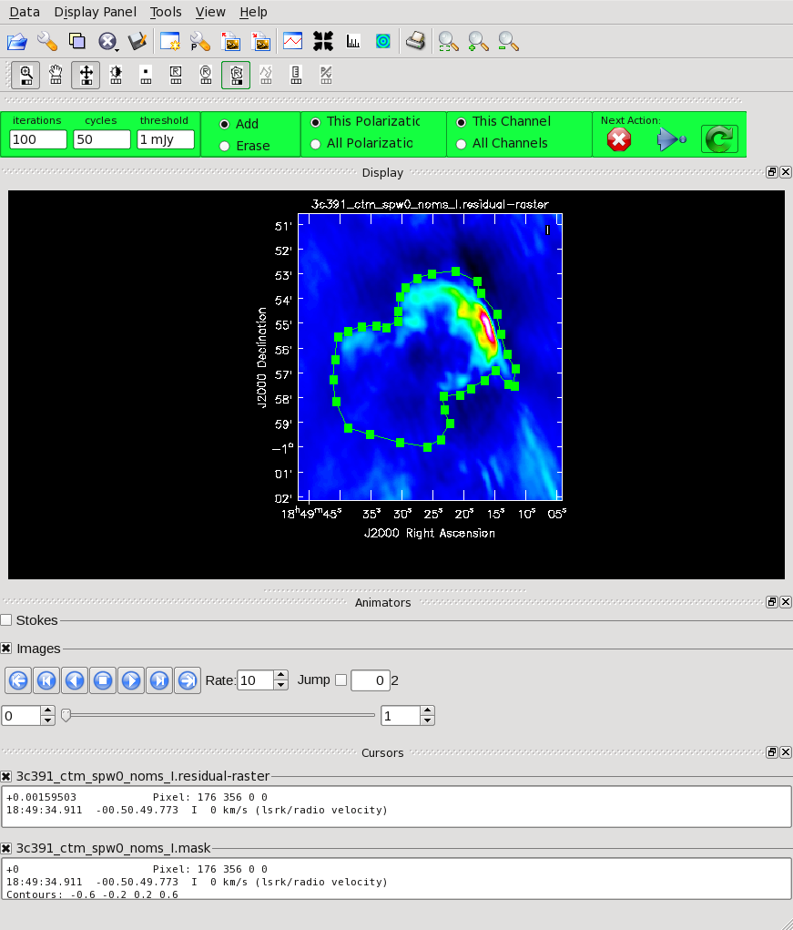
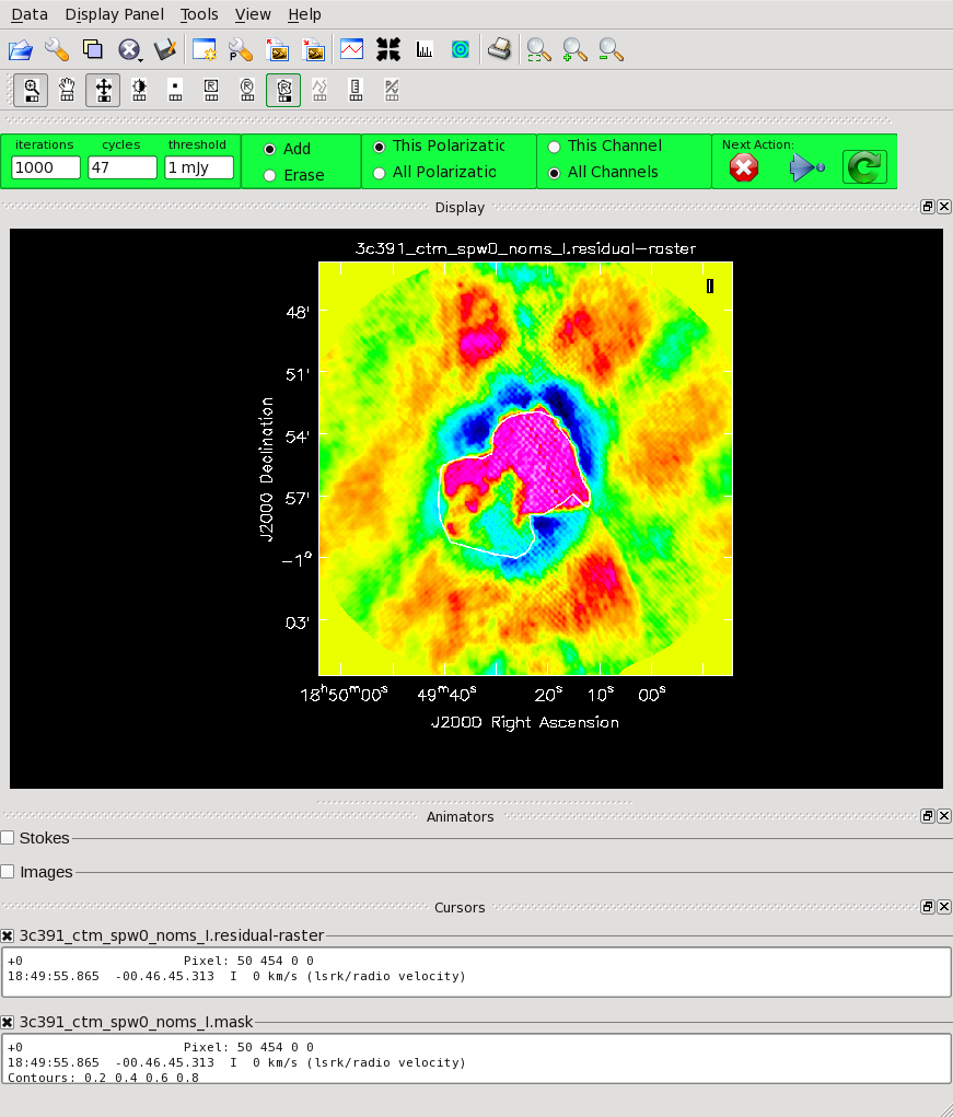
As mentioned above, we can guide the clean process by allowing it to find clean components only within a user-specified region. The easiest way to do this is via interactive clean. When clean runs in interactive mode, a viewer window will pop up as shown right. To get a more detailed view of the central regions containing the emission, zoom in by tracing out a rectangle with the left mouse button and double-clicking inside the zoom box you just made. Play with the color scale to bring out the emission better, by holding down the middle mouse button and moving it around. To create a clean box (a region within which components may be found), hold down the right mouse button and trace out a rectangle around the source, then double click inside that rectangle to set it as a box. Note that the CLEAN box must turn white for it to be registered; if the box is not white, it has not been set! Alternatively, you can trace out a more generic shape to better enclose the irregular outline of the supernova remnant. To do that, right-click on the closed polygonal icon. Then trace out a shape by right-clicking where you want the corners of that shape. Once you have come full circle, the shape will be traced out in green, with small squares at the corners. Double-click inside this region and the green outline will turn white. You have now set the clean region. If you have made a mistake with your clean box, click on the "Erase" button, trace out a rectangle around your erroneous region, and double click inside that rectangle. You can also set multiple clean regions. By default, all clean regions will apply only to the plane shown. To change this to select all planes, click the "All Channels" button at the top (we have only a single mfs channel in the image cube), and likewise for Stokes planes using the "All Polarizations" (you will need to set this when we image all the Stokes).
At any stage in the cleaning, you can adjust the number of iterations that clean will do before returning to the GUI. By default this is set to 100 (see the "iterations" window in mid-upper left of panel). You probably want to set this to a high number for this mosaic due to the complicated structure, values from 1000 to 5000 later on seem to work. Note that this will override the niter that was set when you started the clean task. Clean will keep going until it reaches threshold or runs out of cycles (the "cycles" window to the right of the "iterations").
When you are happy with the clean regions, press the green circular arrow button on the far right to continue deconvolution. After completing a cycle, a revised image will come up. As the brightest points are removed from the image ("cleaned" off), fainter emission may show up. You can adjust the clean boxes each cycle, to enclose all real emission. After many cycles, once only noise is left, you can hit the red and white cross icon to stop cleaning. The second figure to the right shows the interactive clean panel later in the process (after cleaning around 3000 iterations). At this point we have used the polygon tool to draw around the emission. There is still signal left in the residual, and it would take forever to clean all that out using our standard clean! You should just quit after doing around 10000-20000 iterations total. We'll improve this in the next part of the tutorial.
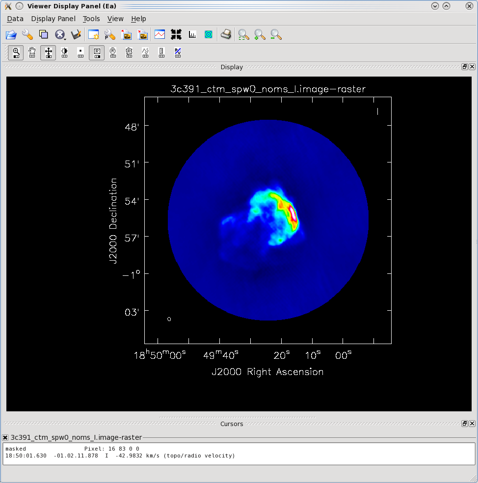
clean will make several output files, all named with the prefix given as imagename. These include:
- .image - final restored image, with the clean components convolved with a restoring beam and added to the remaining residuals at the end of the imaging process
- .flux - effective response of the telescope (the primary beam)
- .flux.pbcoverage - effective response of the full mosaic image
- .mask - areas where clean has been allowed to search for emission
- .model - sum of all the clean components, which also has been stored as the MODEL_DATA column in the measurement set
- .psf - dirty beam, which is being deconvolved from the true sky brightness during the clean process
- .residual - what is left at the end of the deconvolution process; this is useful to diagnose whether or not to clean more deeply
After the imaging and deconvolution process has finished, you can use the viewer to look at your image.
# In CASA
viewer('3c391_ctm_spw0_noms_I.image')
This will bring up a viewer window containing the image, which should look similar to that shown at right. You can adjust the color scale and zoom in to a selected region by assigning mouse buttons to the icons immediately above the image (hover over the icons to get a description of what they do).
Note that the image is cut off in a circular fashion at the edges, corresponding to the default minimum primary beam response (minpb)within clean of 0.2.
As we saw during the interactive cleaning, this single-scale delta-function cleaning is having problems cleaning out the large-scale emission. You can see the large "clean bowl" of negative emission surrounding the object, and the heavy pixelization of the emission at low levels. We'll try to improve on this in the next part of the tutorial.
Continuum Observations Data Reduction Tutorial: 3C 391 - Advanced Topics
Multi-scale Polarization Clean
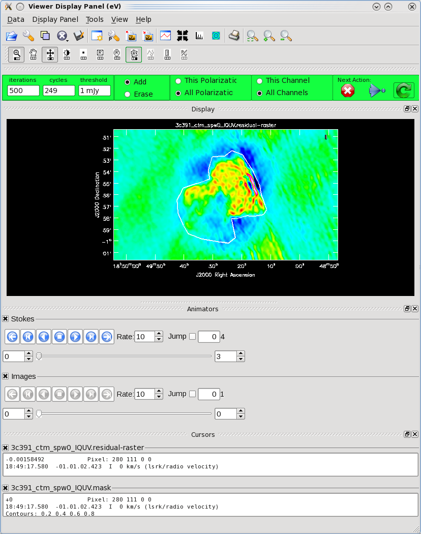
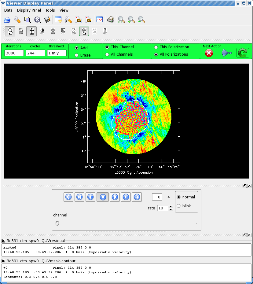
We now employ a multi-scale clean to image Stokes IQUV:
# In CASA
clean(vis='3c391_ctm_mosaic_spw0.ms',imagename='3c391_ctm_spw0_IQUV',
      field='',spw='',
      mode='mfs',
      niter=25000,
      gain=0.1, threshold='1.0mJy',
      psfmode='clarkstokes',
      imagermode='mosaic', ftmachine='mosaic',
      multiscale=[0, 6, 18, 54], smallscalebias=0.9,
      interactive=True,
      imsize=[480,480], cell=['2.5arcsec','2.5arcsec'],
      stokes='IQUV',
      weighting='briggs',robust=0.5,
      pbcor=False,
      usescratch=False)
For these inputs, we have changed:
- stokes='IQUV', psfmode='clarkstokes' : Separate images will be made in all four polarizations (total intensity I, linear polarizations Q and U, and circular polarization V), and, with psfmode='clarkstokes', the Clark CLEAN algorithm will deconvolve each Stokes plane separately thereby making the polarization image more independent of the total intensity.
- multiscale=[0, 6, 18, 54], smallscalebias=0.9 : A multi-scale CLEANing algorithm is used because the supernova remnant contains both diffuse, extended structure on large spatial scales and finer filamentary structure on smaller scales. The settings for multiscale are in units of pixels, with 0 pixels equivalent to the traditional delta-function CLEAN. The scales here are chosen to provide delta functions and then three logarithmically scaled sizes to fit to the data. The first scale (6 pixels) is chosen to be comparable to the size of the beam. The smallscalebias attempts to balance the weight given to larger scales, which often have more flux density, and the smaller scales, which often are brighter. Considerable experimentation is likely to be necessary; one of the authors of this document found that it was useful to CLEAN several rounds with this setting, change to multiscale=[] and remove much of the smaller scale structure, then return to this setting.
- pbcor=False : by default pbcor=False and a flat-noise image is produced. We can do the primary beam correction later (see below).
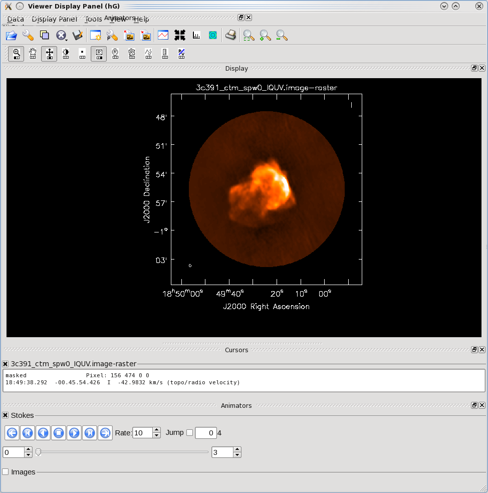
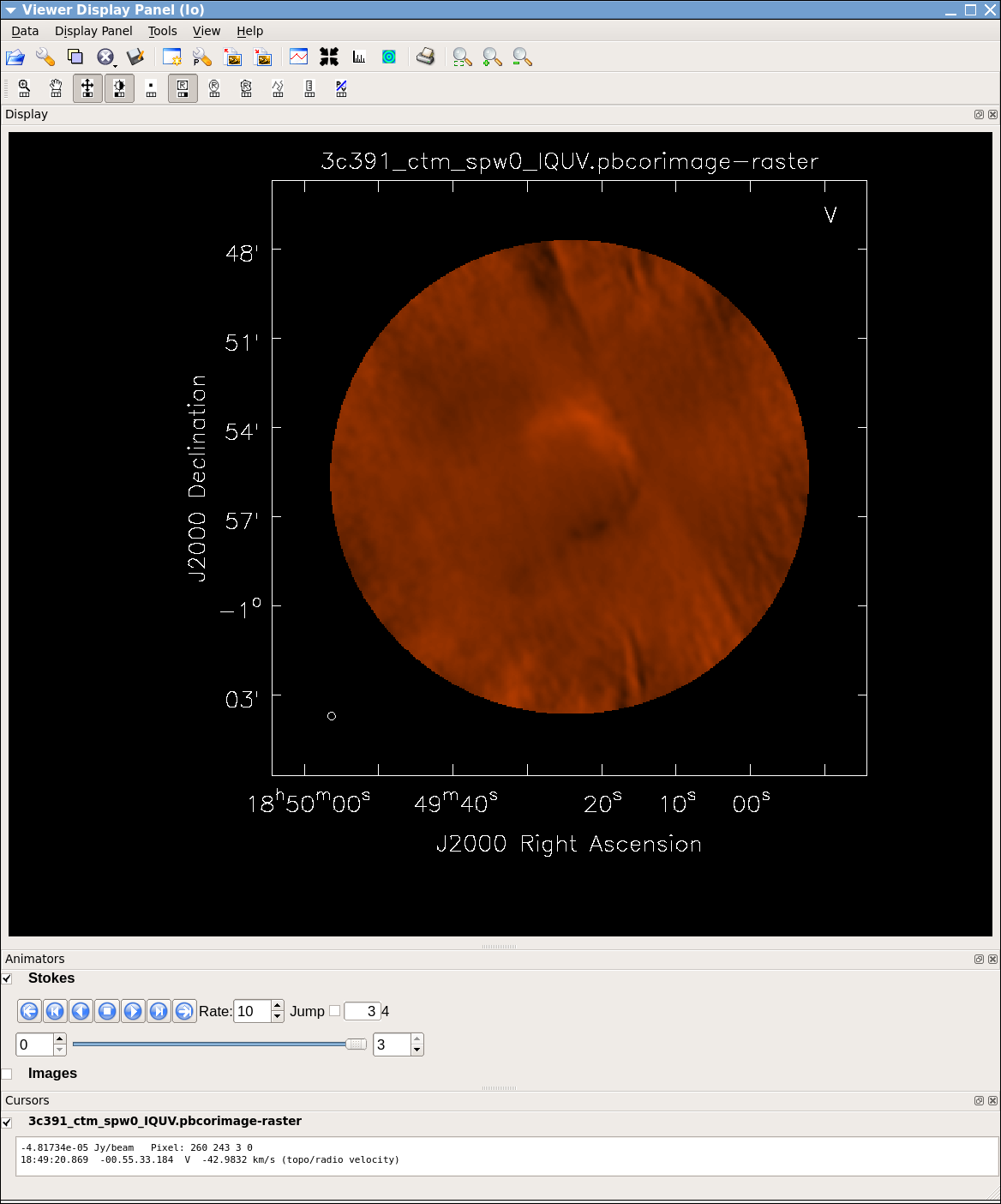
As previously, we guide the clean using polygon regions in the interactive clean GUI. Because we now have the four Stokes planes in the image for IQUV, you should be sure to extend the mask you draw by selecting the "All Polarizations" radio button before drawing the mask. As you clean, you can use the tapedeck to examine the residuals in the QUV planes. In practice, those will reach the 1 mJy threshold fairly quickly and not be cleaned further while the I cleaning proceeds for a long time. In the screen-shots to the right, you can see that the multiscale clean is doing a better job of picking up the larger-scale emission. After about 15000 iterations the residuals were looking pretty good. As mentioned above restarting clean with different multiscale choices can help also.
After the imaging and deconvolution process has finished, you can use the viewer to look at your image.
# In CASA
viewer('3c391_ctm_spw0_IQUV.image')
The tape deck buttons that you see under the image can be used to step through the different Stokes parameters (I,Q,U,V). You can adjust the color scale and zoom in to a selected region by assigning mouse buttons to the icons immediately above the image (hover over the icons to get a description of what they do). Also using the "wrench" panel to change Display Options will be helpful here. In the I Stokes plane (1) shown to the right we chose the "Hot Metal 1" colormap. In the lower panel showing the V Stokes plane (3) we also set the "scaling power cycles" to -1.5 to enhance low-contrast emission. Our Stokes I image is significantly better than with just a delta-function classic clean. You can also explore the Q and U images but we will produce more intuitive images from these later on. Finally, note that the residual emission in Stokes V is not real, but likely due to the EVLA "beam squint" between R and L (they are slightly separated on the sky, and this is not currently compensated for in our production version of clean).
The clean task naturally operates in a "flat noise" image, i.e. an image where the effective weighting across the mosaic field of view is set so that the noise is constant. This is so that the clean threshold has a uniform meaning for the stopping criterion and that the image fed into the minor cycles has uniform noise levels. However, this means that the image does not take into account the primary beam fall-off in the edges and interstices of the mosaic. We could have set pbcor=True in clean, but it is useful to see the flat-noise image and residuals to evaluate the quality of the clean image. Therefore, we use impbcor to divide the .image by the .flux image to produce a primary beam corrected restored image:
# In CASA
impbcor(imagename='3c391_ctm_spw0_IQUV.image',pbimage='3c391_ctm_spw0_IQUV.flux',
        outfile='3c391_ctm_spw0_IQUV.pbcorimage')
You can open this in the viewer and see that it has indeed raised the noise (and signal) at the edges of the mosaic.
Image Analysis and Manipulation
This topic is perhaps not "advanced," but it appears to fit more naturally here. It is assumed that an image 3c391_ctm_spw0_IQUV.image, resulting from the above clean, exists.
The three most basic analyses are to determine the peak brightness, the flux density, and the image noise level. These are useful measures of how well one's imaging efforts are in approaching the thermal noise limit or in reproducing what is already known about a source. Additional discussion of image analysis and manipulation, including the combination of multiple images, mathematical operations on images, and much more can be found in Image Analysis in the CASA Reference Book.
The most straightforward statistic is the peak brightness, which is determined by imstat.
mystat = imstat(imagename='3c391_ctm_spw0_IQUV.pbcorimage',stokes='')
- mystat=imstat() : imstat returns a Python dictionary which we capture in the variable mystat
- stokes=' ' : This example determines the peak brightness in the entire image, which has all four Stokes planes. If one wanted to determine the peak brightness in just, say, the Stokes V image, one would set stokes='V'.
The dictionary contains the values which you can extract for further use. For example, for a particular instance of the previous clean, we found:
CASA <4>: mystat
  Out[4]:
{'blc': array([0, 0, 0, 0], dtype=int32),
 'blcf': '18:50:04.251, -01.05.40.567, I, 4.59901e+09Hz',
 'max': array([ 0.15447657]),
 'maxpos': array([288, 256,   0,   0], dtype=int32),
 'maxposf': '18:49:16.243, -00.55.00.579, I, 4.59901e+09Hz',
 'mean': array([ 0.00081497]),
 'medabsdevmed': array([ 0.00016437]),
 'median': array([  1.00343077e-05]),
 'min': array([-0.00607492]),
 'minpos': array([239, 413,   0,   0], dtype=int32),
 'minposf': '18:49:24.411, -00.48.28.080, I, 4.59901e+09Hz',
 'npts': array([ 481828.]),
 'q1': array([-0.00014913]),
 'q3': array([ 0.00018026]),
 'quartile': array([ 0.0003294]),
 'rms': array([ 0.00590687]),
 'sigma': array([ 0.00585038]),
 'sum': array([ 392.67754914]),
 'sumsq': array([ 16.81150507]),
 'trc': array([479, 479,   3,   0], dtype=int32),
 'trcf': '18:48:44.407, -00.45.43.065, V, 4.59901e+09Hz'}

CASA <5>: mystat['max'][0]
  Out[5]: 0.15447656810283661
and so the peak flux density is 0.154 Jy/beam (likely in the I Stokes plane).
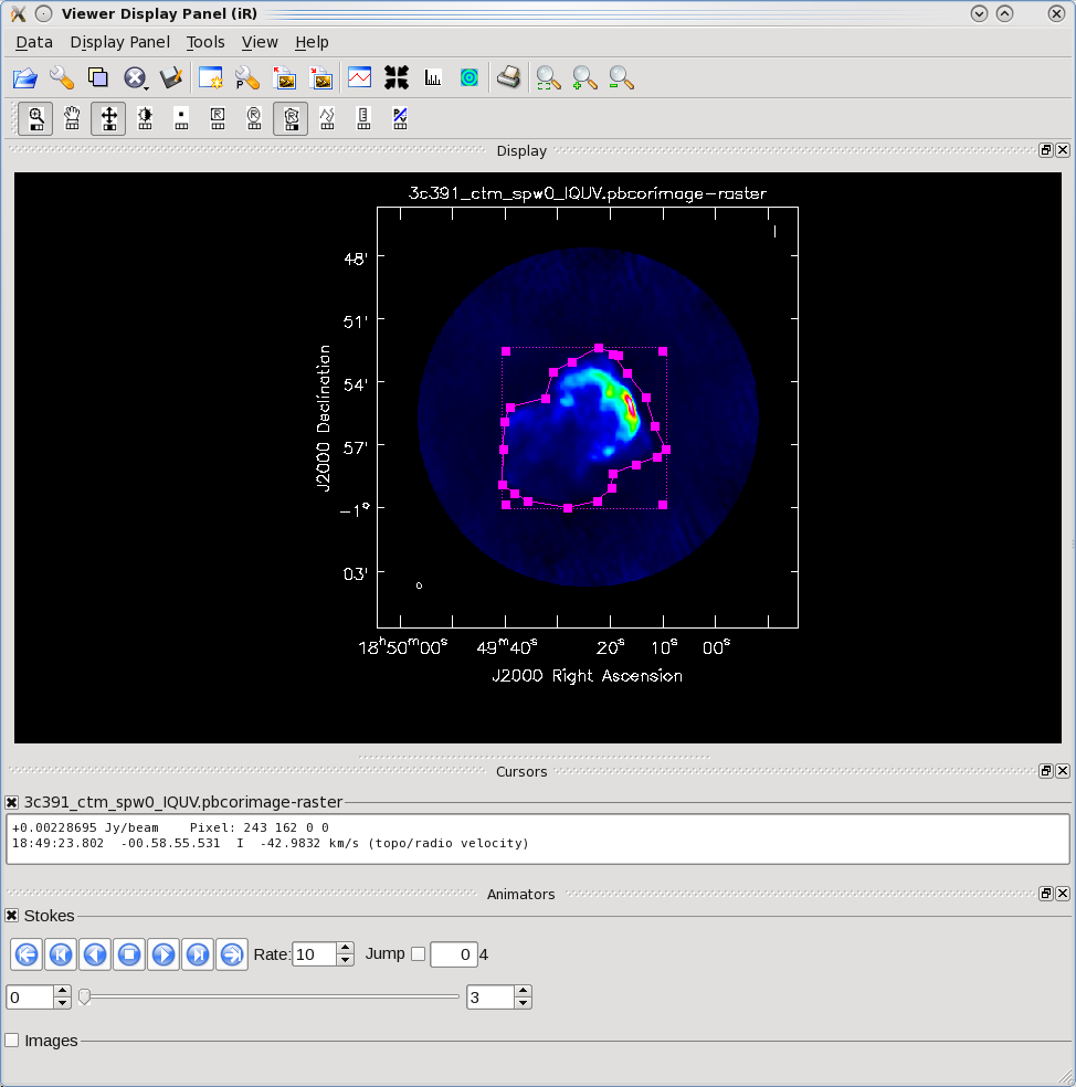
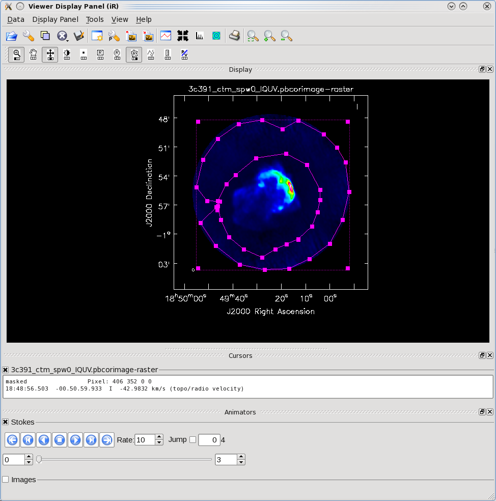
The other two statistics require slightly more care. The flux density of a source is determined by integrating its brightness or intensity over some solid angle, i.e.,
[math]\displaystyle{ S = \int d\Omega I }[/math]
where [math]\displaystyle{ I }[/math] is the intensity (measured in units of Jy/beam), [math]\displaystyle{ \Omega }[/math] is the solid angle of the source (e.g., number of synthesized beams), and [math]\displaystyle{ S }[/math] is the flux density (measured in units of Jy). In general, if the noise is well-behaved in one's image, when averaged over a reasonable solid angle, the noise contribution should approach 0 Jy. If that is the case, then the flux density of the source is also reported by imstat. However, there are many cases for which a noise contribution of 0 Jy may not be a safe assumption. If one's source is in a complicated region (e.g., a star formation region, the Galactic center, near the edge of a galaxy), a better estimate of the source's flux density will be obtained by limiting carefully the solid angle over which the integration is performed.
Open viewer and use it to display the corrected image
# In CASA
viewer('3c391_ctm_spw0_IQUV.pbcorimage')
One can choose the function assigned to each mouse button; after zooming into the desired view, assign 'polygon region' to a desired mouse button (e.g., left button) by selecting the icon shown in the figure to the right with the desired mouse button.
Using the mouse button just assigned to 'polygon region', outline the supernova remnant. You start drawing vertices by clicking on points in the image in succession, when you draw the final vertex then you double-click to connect and close the region. When you mouse is inside the region a bounding box will appear with the vertices shown as draggable solid squares. If you want to adjust the vertices you can do so!
If you find you don't like your region you can dismiss it with with ESC key or using the remove region "X" button in lower right of the panel. You can also employ the region panel to save a region you have created, for later use.
Double click inside of that region (using the same mouse button used to make the region), and the statistics will be reported. This will include the flux density value within the region selected.
 (3c391_ctm_spw0_IQUV.pbcorimage)
        Stokes       Velocity          Frame        Doppler      Frequency
             I   -42.9832km/s           LSRK          RADIO    4.59901e+09
BrightnessUnit       BeamArea           Npts            Sum    FluxDensity
       Jy/beam        45.0996          22203   3.857102e+02   8.552405e+00
          Mean            Rms        Std dev        Minimum        Maximum
  1.737199e-02   2.668837e-02   2.026084e-02  -6.180350e-03   1.528023e-01
  region count
             1
In our example we find a total Flux density of 8.5 Jy while the max brightness is only 0.0173 Jy/beam. Note that the numbers you get may be slightly different depending on how deeply you cleaned.
By contrast, for the rms noise level, one wants load the original (un-pbcor) image
# In CASA
viewer('3c391_ctm_spw0_IQUV.image')
and to exclude the source's emission to the extent possible, as the source's emission will bias the estimated noise level high. Likewise, one should avoid the "clean bowl" around the source emission. One can repeat the procedure above, defining a polygonal region, then double clicking inside it, to determine the statistics. You can use the tapedeck to change which Stokes plane you are viewing and double-click in each to get those statistics. For example, from the region selection shown to the right for off-source statistics:
---- ---- ---- ---- ---- ---- ---- ---- ---- ---- ---- ---- ---- ---- ---- ---- ----
(3c391_ctm_spw0_IQUV.pbcorimage)
        Stokes       Velocity          Frame        Doppler      Frequency
             I   -42.9832km/s           LSRK          RADIO    4.59901e+09
BrightnessUnit       BeamArea           Npts            Sum    FluxDensity
       Jy/beam        45.0996          61753   2.844620e+01   6.307414e-01
          Mean            Rms        Std dev        Minimum        Maximum
  4.606448e-04   1.661159e-03   1.596025e-03  -5.679628e-03   9.719489e-03
  region count
             1
---- ---- ---- ---- ---- ---- ---- ---- ---- ---- ---- ---- ---- ---- ---- ---- ----
---- ---- ---- ---- ---- ---- ---- ---- ---- ---- ---- ---- ---- ---- ---- ---- ----
(3c391_ctm_spw0_IQUV.pbcorimage)
        Stokes       Velocity          Frame        Doppler      Frequency
             Q   -42.9832km/s           LSRK          RADIO    4.59901e+09
BrightnessUnit       BeamArea           Npts            Sum    FluxDensity
       Jy/beam        45.0996          61753  -5.743594e-01  -1.273535e-02
          Mean            Rms        Std dev        Minimum        Maximum
 -9.300915e-06   1.507897e-04   1.505038e-04  -7.758265e-04   8.262882e-04
  region count
             1
---- ---- ---- ---- ---- ---- ---- ---- ---- ---- ---- ---- ---- ---- ---- ---- ----
---- ---- ---- ---- ---- ---- ---- ---- ---- ---- ---- ---- ---- ---- ---- ---- ----
(3c391_ctm_spw0_IQUV.pbcorimage)
        Stokes       Velocity          Frame        Doppler      Frequency
             U   -42.9832km/s           LSRK          RADIO    4.59901e+09
BrightnessUnit       BeamArea           Npts            Sum    FluxDensity
       Jy/beam        45.0996          61753   4.498778e-01   9.975201e-03
          Mean            Rms        Std dev        Minimum        Maximum
  7.285117e-06   1.485673e-04   1.483898e-04  -8.174598e-04   8.751833e-04
  region count
             1
---- ---- ---- ---- ---- ---- ---- ---- ---- ---- ---- ---- ---- ---- ---- ---- ----
---- ---- ---- ---- ---- ---- ---- ---- ---- ---- ---- ---- ---- ---- ---- ---- ----
(3c391_ctm_spw0_IQUV.pbcorimage)
        Stokes       Velocity          Frame        Doppler      Frequency
             V   -42.9832km/s           LSRK          RADIO    4.59901e+09
BrightnessUnit       BeamArea           Npts            Sum    FluxDensity
       Jy/beam        45.0996          61803   2.358344e-01   5.229189e-03
          Mean            Rms        Std dev        Minimum        Maximum
  3.815906e-06   3.209289e-04   3.209089e-04  -1.309853e-03   1.316741e-03
  region count
             1
---- ---- ---- ---- ---- ---- ---- ---- ---- ---- ---- ---- ---- ---- ---- ---- ----
Thus the I rms is 1.6 mJy and Q and U rms are around 0.15 mJy. It will be useful later on to have the flat-noise and pb-corrected images available separately along with the statistics.
Constructing Polarization Intensity and Angle Images
At the beginning of this Advanced Tutorial, a full polarization imaging cube of 3C 391 was constructed. This cube has 3 dimensions, the standard two angular dimensions (right ascension, declination) and a third dimension containing the polarization information. Considering the image cube as a matrix, [math]\displaystyle{ Image[l,m,p] }[/math], the [math]\displaystyle{ l }[/math] and [math]\displaystyle{ m }[/math] axis describe the sky brightness or intensity for the given [math]\displaystyle{ p }[/math] axis. If one opens the viewer and loads the 3C 391 continuum image, the default view contains an "animator" or pane with movie controls. One can step through the polarization axis, displaying the images for the different polarizations.
As created, the image contains four polarizations, for the four Stokes parameters, I, Q, U, and V. Recalling the lectures, Q and U describe the linear polarization and V describes the circular polarization. Specifically, Q describes the amount of linear polarization aligned with a given axis, and U describes the amount of linear polarization at a 45 deg angle to that axis. The V parameter describes the amount of circular polarization, with the sign (positive or negative) describing the sense of the circular polarization (right- or left-hand circularly polarized).
In general, few celestial sources are expected to show circular polarization, with the notable exception of masers, while terrestrial and satellite sources are often highly circularly polarized. The V image is therefore often worth forming because any V emission could be indicative of unflagged RFI within the data (or problems with the calibration!).
Because the Q and U images both describe the amount of linear polarization, it is more common to work with a linear polarization intensity image, [math]\displaystyle{ P = \sqrt{Q^2 +U^2} }[/math]. ([math]\displaystyle{ P }[/math] can also be denoted by [math]\displaystyle{ L }[/math].) Also important can be the polarization position angle [math]\displaystyle{ tan 2\chi = U/Q }[/math].
The relevant task is immath, with specific examples for processing of polarization images given in Polarization Manipulation. The steps are the following.
1. Extract the I, Q, U, V planes from the full Stokes image cube, forming separate images for each Stokes parameter. Use the flat-noise images so that non-uniform noise does not bias us.
# In CASA
immath(imagename='3c391_ctm_spw0_IQUV.image',outfile='3c391_ctm_spw0.I',expr='IM0',stokes='I')
immath(imagename='3c391_ctm_spw0_IQUV.image',outfile='3c391_ctm_spw0.Q',expr='IM0',stokes='Q')
immath(imagename='3c391_ctm_spw0_IQUV.image',outfile='3c391_ctm_spw0.U',expr='IM0',stokes='U')
immath(imagename='3c391_ctm_spw0_IQUV.image',outfile='3c391_ctm_spw0.V',expr='IM0',stokes='V')
We also extract a pb-corrected I image for later use:
# In CASA
immath(outfile='3c391_ctm_spw0.pbcorI',
       mode='evalexpr',
       imagename='3c391_ctm_spw0_IQUV.pbcorimage',
       expr='IM0',stokes='I')
2. Combine the Q and U images using the mode='poli' option of immath to form the linear polarization image.
# In CASA
immath(outfile='3c391_ctm_spw0.P',
       mode='poli',
       imagename=['3c391_ctm_spw0.Q','3c391_ctm_spw0.U'],
       sigma='0.0Jy/beam')
Because P is formed from the sum of the squares of the Q and U values, it is biased by the noise. In principle, one can set the sigma value to debias this (it subtracts the square of this value from the Q2+U2 before taking the square-root).
# In CASA
immath(outfile='3c391_ctm_spw0.P_unbias',
       mode='poli',
       imagename=['3c391_ctm_spw0.Q','3c391_ctm_spw0.U'],
       sigma='0.000041Jy/beam')
Currently in CASA 4.1 and earlier, there is a bug where pixels where the noise subtraction makes it negative are set to NaN. To filter this out use immath. Also, you must give sigma in Jy/beam (not mJy/beam). We do:
# In CASA
immath(outfile='3c391_ctm_spw0.P_unbias_filtered',
       mode='evalexpr',
       imagename=['3c391_ctm_spw0.P_unbias'],
       expr="IM0[IM0>-10000.0]")
Finally, one can pb-correct this (after first extracting one plane of the .flux image, they are all the same):
# In CASA
immath(imagename='3c391_ctm_spw0_IQUV.flux',
       outfile='3c391_ctm_spw0.Qflux',
       expr='IM0',stokes='Q')
#
immath(outfile='3c391_ctm_spw0.pbcorP',
       mode='evalexpr',
       imagename=['3c391_ctm_spw0.P_unbias_filtered','3c391_ctm_spw0.Qflux'],
       expr="IM0[IM1>0.2]/IM1")
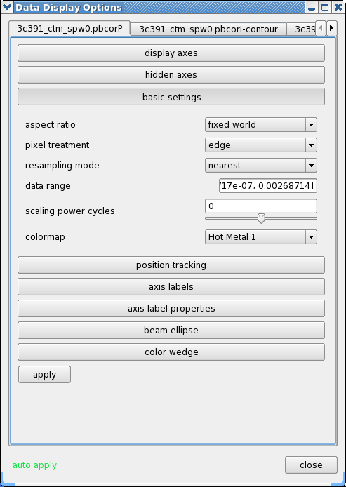
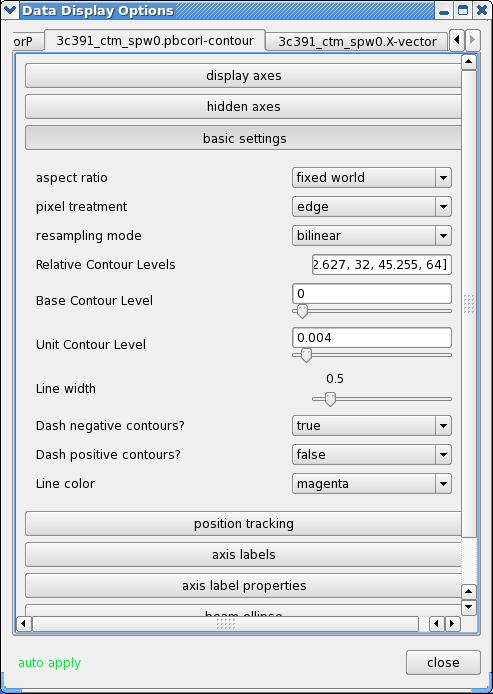
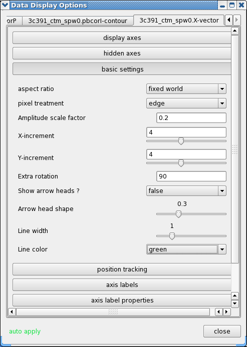
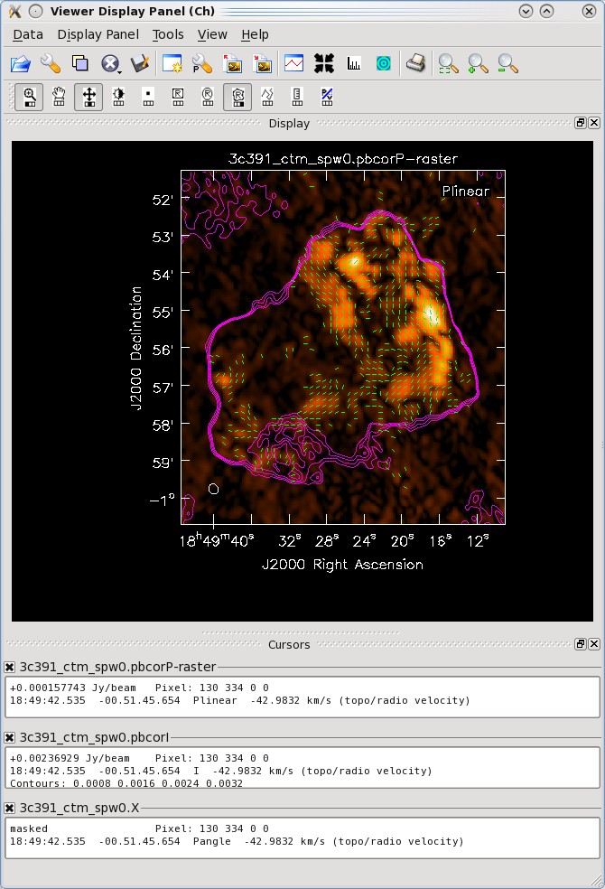
3. Combine the Q and U images using the mode='pola' option of immath to form the polarization position angle image. Because the polarization position angle is derived from the tangent function, the order in which the Q and U images are specified is important. Also, we use the flat-noise images as only the ratio matters and for thresholding you want a uniform noise:
# In CASA
immath(outfile='3c391_ctm_spw0.X',
       mode='pola',
       imagename=['3c391_ctm_spw0.Q','3c391_ctm_spw0.U'],
       polithresh='0.2mJy/beam')
To avoid displaying the position angle of noise, we can set a threshold intensity of the linear polarization for above which we wish to calculate the polarization angle, using the polithresh parameter. An appropriate level here might be the [math]\displaystyle{ 5\sigma }[/math] level of around 0.2 mJy/beam.
4. If desired, form the fractional linear polarization image, defined as P/I. We can do this on the flat-noise image.
# In CASA
immath(outfile='3c391_ctm_spw0.F',
       mode='evalexpr',
       imagename=['3c391_ctm_spw0.I','3c391_ctm_spw0.Q','3c391_ctm_spw0.U'],
       expr='sqrt((IM1^2+IM2^2)/IM0[IM0>1.2e-3]^2)')
Since the total intensity image can (and hopefully does) approach zero in regions free of source emission, dividing by the total intensity can produce very high pixel values in these regions. We therefore wish to restrict our fractional polarization image to regions containing real emission, which we do by setting a threshold in the total intensity image, which in this case corresponds to three times the I noise level. The computation of the polarized intensity is specified by
expr='sqrt((IM1^2+IM2^2)/IM0[IM0>1.2e-3]^2)'
with the expression in square brackets setting the threshold in IM0 (the total intensity image). Note that IM0, IM1 and IM2 correspond to the three files listed in the imagename array, in that order. The order in which the different images are specified is therefore critical once again.
One can then view these various images using viewer. It is instructive to display the I, P and X images (total intensity, total linearly polarized intensity, and polarization position angle) together, to show how the polarized emission relates to the total intensity, and how the magnetic field is structured. We can do this using the viewer.
- Begin by loading the linear polarization image in the viewer:
# In CASA
viewer('3c391_ctm_spw0.pbcorP')
- Next, load the pb-corrected total intensity image as a contour image. In the viewer panel, hit the "Open" icon (the leftmost button in the top row of icons in the viewer). This will bring up a 'Load Data' GUI showing all images and MS in the current directory. Select the total intensity image (3c391_ctm_spw0.pbcorI) and click the 'Contour Map' button on the right hand side.
- Finally, load the polarization position angle image (3c391_ctm_spw0.X) as a vector map.
While we set the polithresh parameter when we created the position angle (X) image, a digression here is instructive in the use of LEL Expressions. Had we not set this parameter, the position angle would have been derived for all pixels within the full IQUV image cube. There is only polarized emission from a limited subset of pixels within this image. Therefore, to avoid plotting vectors corresponding to the position angle of pure noise, we would now wish to select only the regions where the polarized intensity is brighter than some threshold value. To do this, we would use a LEL (Lattice Expression Language) Expression in the 'Load Data' GUI. For our chosen threshold of 0.4 mJy (the 5 sigma level in the pbcorP image), we would paste the expression
'3c391_ctm_spw0.X'['3c391_ctm_spw0.pbcorP'>0.0004]
into the LEL Expression box in the GUI, and click the 'Vector Map' button. This would load the vectors only for regions where [math]\displaystyle{ P\gt 0.4 }[/math] mJy.
While we now have all three images loaded into the viewer (the polarized intensity (3c391_ctm_spw0.pbcorP) in color, the total intensity (3c391_ctm_spw0.pbcorI) as a contour map, and the polarization position angle (3c391_ctm_spw0.X) as a vector map), we still wish to optimize the display for ease of interpretation.
- Click the wrench icon to open a 'Data Display Options' GUI. This will have 3 tabs, corresponding to the three images loaded.
- Change the image transfer function. Hold down the middle mouse button and move the mouse until the color scale is optimized for the display of the polarized intensity. You can change the colormap (e.g. to HotMetal1) in the first tab of the Data Display Options GUI.
- Change the contour levels. Select the total intensity tab (3c391_ctm_spw0.pbcorI) tab (2nd) in the Data Display Options GUI. Change the relative contour levels from the default levels of [0.2,0.4,0.6,0.8,1.0] to powers of [math]\displaystyle{ \sqrt{2} }[/math], including a couple of negative contours at the beginning to demonstrate the image quality. An appropriate set of levels might be [-1.414,-1,1,1.414,2,2.828,4,5.657,8,11.314,16,22.627,32,45.255,64]. These levels will multiply the Unit Contour Level, which we set at some multiple of the rms noise in the total intensity image. An appropriate value might be 0.004 Jy ([math]\displaystyle{ 5\sigma }[/math] of pbcorI rms in the outer part of the mosaic). Choose a nice contour color (e.g. "magenta").
- Change the vector spacing and color, and rotate the vectors. The polarization position angle as calculated is the electric vector position angle (EVPA). If we are interested in the orientation of the magnetic field, then for an optically thin source, the magnetic field orientation is perpendicular to the EVPA, so we must rotate the vectors by [math]\displaystyle{ 90^{\circ} }[/math]. Select the vector image tab in the 'Data Display Options' GUI (labeled as the LEL expression we entered in the Load Data GUI) and enter 90 in the Extra rotation box. If the vectors appear too densely packed on the image, change the spacing of the vectors by setting X-increment and Y-increment to a larger value (4 might be appropriate here). Finally, to be able to distinguish the vectors from the total intensity contours, change the color of the vectors by selecting a different Line color (green might be a good choice).
Now that we have altered the display to our satisfaction, it remains only to zoom in to the region containing the emission. Close the animator tab in the viewer, and then drag out a rectangular region around the supernova remnant with your left mouse button. Double-click to zoom in to that region. This will give you a final image looking something like that shown at right.
Spectral Index Imaging
The spectral index, defined as the slope of the radio spectrum between two different frequencies, [math]\displaystyle{ \log(S_{\nu_1}/S_{\nu_2})/\log(\nu_1/\nu_2) }[/math], is a useful analytical tool which can convey information about the emission mechanism, the optical depth of the source or the underlying energy distribution of synchrotron-radiating electrons.
Having used immath to manipulate the polarization images, the reader should now have some familiarity with performing mathematical operations within CASA. immath also has a special mode for calculating the spectral index, mode='spix' . The two input images at different frequencies should be provided using the parameter (in this case, the Python list) imagename. With this information, it is left as an exercise for the reader to create a spectral index map.
The two input images could be the two different spectral windows from the 3C391 continuum data set (see below). If the higher-frequency spectral window (spw1) has not yet been reduced, then two images made with different channel ranges from the lower spectral window, spw0, should suffice. In this latter case, the extreme upper and lower channels are suggested, to provide a sufficient lever arm in frequency to measure a believable spectral index.
Note: It would be desirable to produce the spectral index image through the first-order Taylor term expansion in the MFS imaging. This is unfortunately not available with mosaics in the current version of CASA. Stay tuned.
Self-Calibration
Recalling the lectures, even after the initial calibration using the amplitude calibrator and the phase calibrator, there are likely to be residual phase and/or amplitude errors in the data. Self-calibration is the process of using an existing model, often constructed by imaging the data itself. Provided that sufficient visibility data have been obtained, and this is essentially always the case with the EVLA (and often the VLBA, and should be with ALMA), the system of equations is wildly over-constrained for the number of unknowns.
More specifically, the observed visibility data on the [math]\displaystyle{ i }[/math]-[math]\displaystyle{ j }[/math] baseline can be modeled as
[math]\displaystyle{ V'_{ij} = G_i G^*_j V_{ij} }[/math]
where [math]\displaystyle{ G_i }[/math] is the complex gain for the [math]\displaystyle{ i^{\mathrm{th}} }[/math] antenna and [math]\displaystyle{ V_{ij} }[/math] is the "true" visibility. For an array of [math]\displaystyle{ N }[/math] antennas, at any given instant, there are [math]\displaystyle{ N(N-1)/2 }[/math] visibility data, but only [math]\displaystyle{ N }[/math] gain factors. For an array with a reasonable number of antennas, [math]\displaystyle{ N }[/math] >~ 8, solutions to this set of coupled equations converge quickly.
There is a small amount of discussion in the CASA Reference Manual on self calibration, but we have lectures on Self-calibration given at NRAO community days. In self-calibrating data, it is useful to keep in mind the structure of a Measurement Set: there are three columns of interest for an MS, the DATA column, the MODEL column, and the CORRECTED_DATA column. In normal usage, as part of the initial split, the CORRECTED_DATA column is set equal to the DATA column. The self-calibration procedure is then
- Produce an image (clean) using the CORRECTED_DATA column.
- Derive a series of gain corrections (gaincal) by comparing the DATA columns and the Fourier transform of the image, which is stored in the MODEL column. These corrections are stored in an external table.
- Apply these corrections (applycal) to the DATA column, to form a new CORRECTED_DATA column, overwriting the previous contents of CORRECTED_DATA.
The following example begins with the standard data set, 3c391_ctm_mosaic_spw0.ms, resulting from the steps above. From this we will make an I-only multiscale image (3c391_ctm_spw0_I.image) and in particular the model (3c391_ctm_spw0_I.model) to generate a series of gain corrections (stored in 3C391_ctm_mosaic_spw0.selfcal1), those gain corrections are applied to the data to form a set of self-calibrated data, and new image is then formed (3c391_ctm_spw0_IQUV_selfcal1.image). Note that in the clean before the self-cal, it is important that we only image I so that any cleaned polarization does not affect the gaincal. Note that in CASA 4.0 we first use delmod on the MS to get rid of the previous polarized model.
#In CASA
delmod('3c391_ctm_mosaic_spw0.ms')
#
clean(vis='3c391_ctm_mosaic_spw0.ms',imagename='3c391_ctm_spw0_ms_I',
      field='',spw='',
      mode='mfs',
      niter=25000,
      gain=0.1,threshold='1mJy',
      psfmode='clark',
      imagermode='mosaic',ftmachine='mosaic',
      multiscale=[0, 6, 18, 54],smallscalebias=0.9,
      interactive=True,
      imsize=[480,480],cell=['2.5arcsec','2.5arcsec'],
      stokes='I',
      weighting='briggs',robust=0.5,
      usescratch=False)
You don't (or even shouldn't) have to clean extremely deep. You want to be sure to capture as much of the source total flux density as possible, but not include low-level questionable features or sub-structure (ripples) that might be due to calibration or clean artifacts.
After you are happy with the image:
#In CASA
gaincal(vis='3c391_ctm_mosaic_spw0.ms',caltable='3c391_ctm_mosaic_spw0.selfcal1',
        field='',spw='',selectdata=False,
        solint='30s',refant='ea21',minblperant=4,minsnr=3,
        gaintype='G',calmode='p',append=False)
#
applycal(vis='3c391_ctm_mosaic_spw0.ms',
         field='',spw='',selectdata=False,
         gaintable= ['3c391_ctm_mosaic_spw0.selfcal1'],gainfield=[''],interp=['nearest'],
         calwt=[False],applymode='calflag')
The CORRECTED_DATA column of the MS now contains the self-calibrated visibilities, when will now be used by clean. Note that the gaincal step will report a number of solutions with insufficient SNR. By default with applymode='calflag' data with no good solutions will be flagged by applycal, in this case you will see it report the flagged fraction increasing from 28% to 43%. This may or may not be a good thing. You can control the action of applycal in this regard by changing the value of applymode: setting applymode='calflagstrict' will be even more stringent about flagging things without valid calibration, while applymode='calonly' will calibrate those with solutions while passing through data without unchanged. Note that you can see ahead of time what applycal will do by running with applymode='trial' which will do the reporting but nothing else.
Questions for the Advanced Student:
|
If you planned on doing multiple iterations of self-cal, you would do another I-only image (e.g. 3c391_ctm_spw0_ms_I_selfcal1) as that is what is needed for the next step. If you want to just go ahead and see what this selfcal has done, make a full IQUV cube:
#In CASA
clean(vis='3c391_ctm_mosaic_spw0.ms',imagename='3c391_ctm_spw0_IQUV_selfcal1',
      field='',spw='',
      mode='mfs',
      niter=25000,
      gain=0.1,threshold='1mJy',
      psfmode='clarkstokes',
      imagermode='mosaic',ftmachine='mosaic',
      multiscale=[0, 6, 18, 54],smallscalebias=0.9,
      interactive=True,
      imsize=[480,480],cell=['2.5arcsec','2.5arcsec'],
      stokes='IQUV',
      weighting='briggs',robust=0.5,
      usescratch=False)
Questions for the Advanced Student:
|
Commonly, this procedure is applied multiple times. The number of iterations is determined by a combination of the data quality and number of antennas in the array, the structure of the source, the extent to which the original self-calibration assumptions are valid, and the user's patience. With reference to the original self-calibration equation above, if the observed visibility data cannot be modeled well by this equation, no amount of self-calibration will help. A not-uncommon limitation for moderately high dynamic range imaging is that there may be baseline-based factors that modify the "true" visibility. If the corruptions to the "true" visibility cannot be modeled as antenna-based, as they are above, self-calibration won't help.
Self-calibration requires experimentation. Do not be afraid to dump an image, or even a set of gain corrections, change something and try again. Having said that, here are several general comments or guidelines:
- Bookkeeping is important! Suppose one conducts 9 iterations of self-calibration. Will it be possible to remember one month later (or maybe even one week later!) which set of gain corrections and images are which? In the example above, the descriptor 'selfcal1' is attached to various files to help keep straight which is what. Successive iterations of self-cal could then be 'selfcal2', 'selfcal3', etc.
- Care is required in the setting of imagename. If one has an image that already exists, CASA will continue CLEANing it (if it can), which is almost certainly not what one wants during self-calibration. Rather one wants a unique imagename for each pass of self-calibration.
- A common metric for whether self-calibration is whether the image dynamic range (= max/rms) has improved. An improvement of 10% is quite acceptable.
- Be careful when making images and setting CLEAN regions or masks. Self-calibration assumes that the model is "perfect." If one CLEANs a noise bump, self-calibration will quite happily try to adjust the gains so that the CORRECTED_DATA describe a source at the location of the noise bump. As the author demonstrated to himself during the writing of his thesis, it is quite possible to take completely noisy data and manufacture a source. It is far better to exclude some feature of a source or a weak source from initial CLEANing and conduct another round of self-calibration than to create an artificial source. If a real source is excluded from initial CLEANing, it will continue to be present in subsequent iterations of self-calibration; if it's not a real source, one probably isn't interested in it anyway.
- Start self-calibration with phase-only solutions (calmode='p' in gaincal). As Rick Perley has discussed in previous summer school lectures, a phase error of 20 deg is as bad as an amplitude error of 10%.
- In initial rounds of self-calibration, consider solution intervals longer than the nominal sampling time (solint in gaincal) and/or lower signal-to-noise ratio thresholds (minsnr in gaincal). Depending upon the frequency and configuration and fidelity of the model image, it can be quite reasonable to start with solint='30s' or solint='60s' and/or minsnr=3 (or even lower). One might also want to consider specifying a uvrange, if, for example, the field has structure on large scales (small [math]\displaystyle{ u }[/math]-[math]\displaystyle{ v }[/math]) that is not well represented by the current image.
- The task applycal will flag data with no good calibration solutions. During the initial self-calibration steps, this flagging may be excessive. If so, one can restore the flags to the state right before running applycal by using the task flagmanager.
- One can track the agreement between the DATA, CORRECTED_DATA, and MODEL in plotms. The options in 'Axes' allows one to select which column is to be plotted. If the MODEL agrees well with the CORRECTED_DATA, one can use shorter solint and/or higher minsnr values.
- One should consider examining the solutions from gaincal, using plotcal, in order to assure one's self that the corrections are sensible. Smoothly varying phases are good, jumps are usually not. (However, because the phases are often plotted +/- 180 degrees, there can be apparent "jumps," if the phases are very near +180 deg or -180 deg.)
- In the case of a mosaic, such as here, one should also verify that the solutions are of equal quality for all of the fields.
On Your Own: 3C391 second frequency and G93.3+6.9
Now that you have run through spw 0 of 3C391, you are ready to strike off on your own with other datasets. We have provided two options here, described below. The first option is simplest as it is the same object (different spectral window). But for a more rewarding challenge try the L-band dataset on G93.3+6.9!
You can find the data in the CASA repository. Both datasets are contained in this "tarball". Note that these MSes do not have the scratch columns pre-made (to keep the sizes small) so you can do an inintial clearcal to force the creation (or wait until you first calibration task does it for you).
1. 3C391 spw 1 (at 7.5 GHz)
This is the second spectral window split off from the 3C391 dataset. You can process this as you did the first, but beware of RFI in this band! You will have to avoid it (through channel ranges) and/or edit it out. Once you have processed this data and imaged it, you can combine those images in immath to make a spectral index image (see above), or combine the two calibrated MSes in clean to make a deeper MFS image (this might be tricky). You can also look for signs of Faraday Rotation by searching for a polarization angle change between the two spw. Can you derive the "rotation measure" (RM)?
2. Supernova Remnant G93.3+6.9 at L-band
This is data taken at L-band of an entirely different Supernova Remnant, centered near 1400 MHz. You should be able to process this data in a very similar manner to the C-band data on 3C391. Note that we are not telling you what you will see in the image ahead of time - you'll have to try it to see! Here are some data reduction hints to help you along:
- There is strong RFI in this spectral window of the original 2 spw dataset. You will need to find it (e.g. using plotms) and avoid it in imaging. You can also flag those channels using flagdata, but this is not necessary. Note that there is a single baseline that shows very strong interference, see if you can find it! You can flag it using the baseline syntax in flagdata (e.g. antenna='ea0x&ea0y').
- We have not edited out bad or dead antennas for you (unlike in 3C391). You will need to find these using plotms and then flagdata them. One helpful plotms trick is to set antenna='ea01' and pick a few channels (like spw='0:30~33') and a single scan (e.g. scan='2~3') and plot the amp versus Antenna2 on the x-axis. You should see the bad antennas (the low ones). As a check set antenna='ea02' and repeat. Is it the same?
- In spite of RFI, the antenna-based calibration is remarkably resilient to moderate to low RFI contamination (which tends to be baseline-based). So rather than flagging channels with RFI, you might try going ahead with calibration and seeing if the solutions make sense. We were able to calibrate this data without flagging channels (only getting the bad baseline noted above).
- There is no observation of a flux or polarization angle calibrator like J1331+3030. You need to use setjy to set the I flux of the gain calibrator. We use the approximate flux density of 5.8 Jy for J2038+5119.
- When it comes time to calibrate the polarization leakage, we are in good shape since J2038+5119 was observed through a range of parallactic angle (use plotms to plot versus ParAngle). Use poltype='Df+QU' to solve for leakage and the unknown polarization of this source. We do not know the true polarization angle of this source, so before doing poltype='Xf' use setjy to set the Q flux to 5.8Jy * fractional pol (determined in leakage polcal run). This will at least align the polarization when you image it.
- The L-band field of view is much larger than at C-band. From the VLA Observational Status Summary (OSS) the resolution should be around 45" in D-config. Use a cellsize of 15" or smaller. What is the primary beam of the VLA at 1.4MHz? How big should you make your image?
- As you clean you will see faint sources all over the field. Welcome to L-band imaging! This SNR has lots of structure - try both standard and multi-scale clean.
Last checked on CASA Version 4.5.2