VLA 5 GHz continuum survey of Seyfert galaxies 5.7.2

↵ VLA Tutorials

This particular tutorial demonstrates how to calibrate a VLA continuum survey, consisting of a flux calibrator, target sources, and their respective phase calibrators. What distinguishes this example is that it includes multiple sources and multiple phase calibrators.

Importing VLA Archive Data

Download your data from the VLA Archive; in this example we'll use the publicly available survey AG733, which consists of VLA C-array, C-band (5 GHz) continuum observations of a handful of Seyfert galaxies.

With some sensible fiddling of the web interface, you should be able to download two archive formatted files, with names like AG733_A061209.xp1 and AG733_B061213.xp1.

Example snippet of listobs output for program AG733.

It's helpful to make a subdirectory to store the VLA archive data and the CASA measurement sets before starting CASA. Linux-level commands are given assuming you are using bash as your default shell.

# In bash
mkdir ~/AG733
mv AG733_? ~/AG733
cd ~/AG733
casapy

To load the data in CASA, we employ the importvla command.

Graphics window produced by plotants. Shown are the antennas of the VLA for the program AG733.

# In CASA
# Before importing, get rid of any original version of the measurement set
if os.path.exists('ag733.ms'): rmtables('ag733.ms')
# let glob find the archive files, store in a python global "myFiles"
from glob import glob as filesearch 
myFiles = filesearch("AG733*.xp?")
importvla(archivefiles=myFiles,vis='ag733.ms')
listobs('ag733.ms')
vishead('ag733.ms')

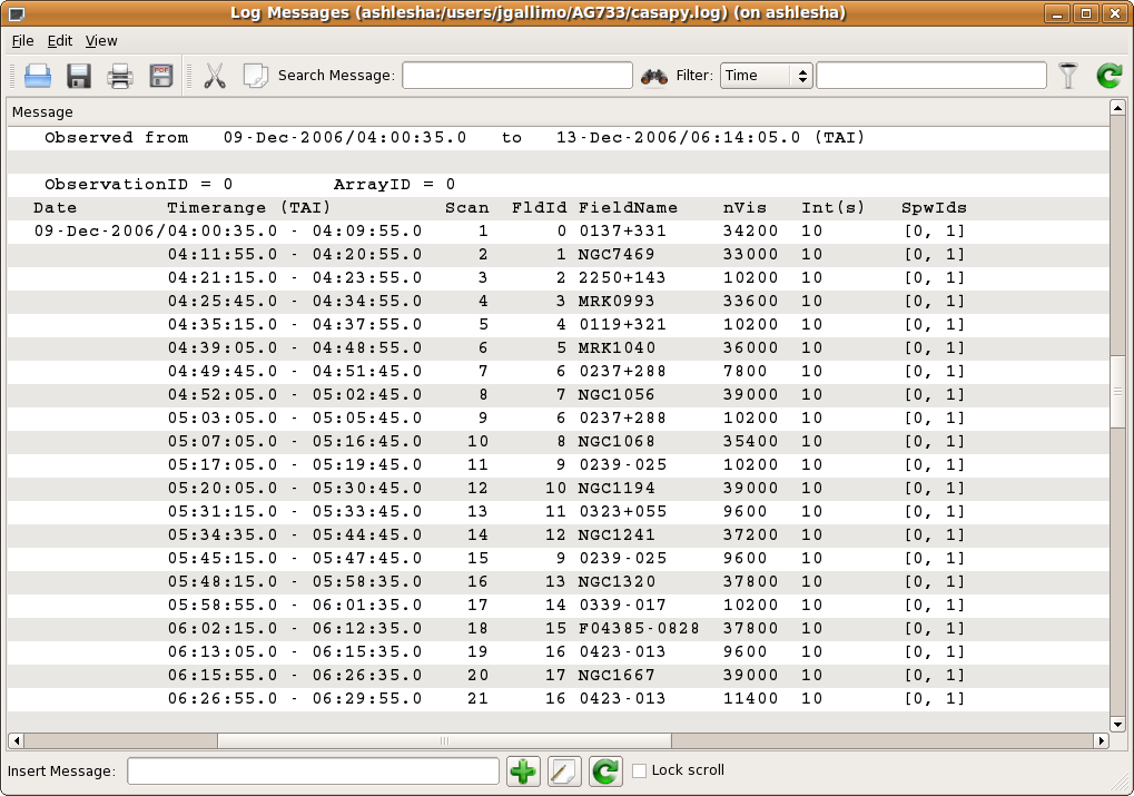
The output measurement set, i.e., the data to be worked on, is ag733.ms. Note that the (interesting) output of listobs and vishead go to the CASA message log window.

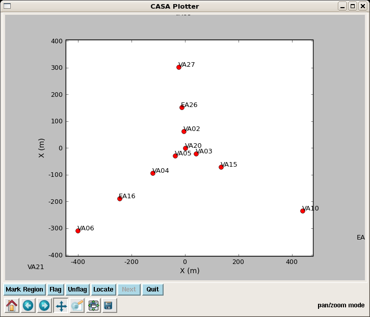
Listobs is similar to LISTR in AIPS and provides a list of scans, sources and their respective indices, and antennas. You can also get a more useful plot of antennas, akin to the output of the AIPS task PRTAN, using plotants. The antennas plot aids the selection of a reference antenna; the antenna VA05 looks like a reasonable choice.

# In CASA
vis = 'ag733.ms'
plotants()

Beta-alert: At the time of this revision (CASA 3.2), plotants was leaving table.lock files that make the rest of the tutorial unhappy. Here's a pythonic way to zap those table.lock files.

import os
for root, dirs, files in os.walk('./'):
    for name in files:
        if name == 'table.lock': os.remove(os.path.join(root,name))

Editing the Measurement Set

This technique is detailed in the tutorial Data flagging with plotms. Here's a shorter version.

# In CASA
plotms()

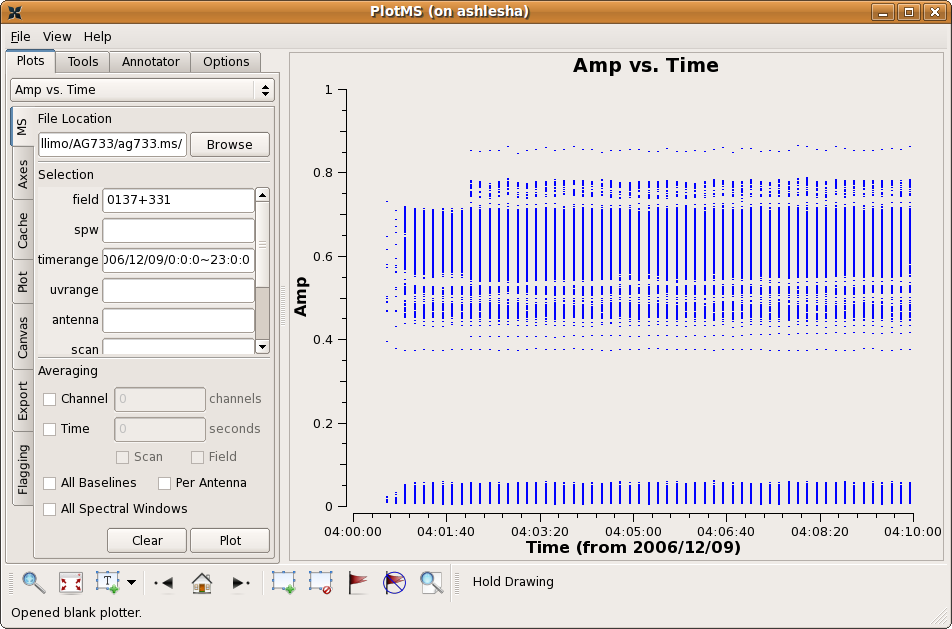
Plotms brings up the following graphical display.

In this example, the measurement set was selected by navigating to and highlighting the measurement set ag733.ms (which will look like a directory to your file browser, but only because it is a directory). A specific subset of data (the flux calibrator 3C48 = 0137+331 on the first observing day) was selected by specifying in the appropriate filter boxes,

field = '0137+331', and
timerange = 2006/12/09/0:0:0~23:0:0.

In the example shown, the data were already edited. No obviously bad data remain. Note that the low points are actually cross-polarization data; at the time of this writing, plotms (in beta) could not yet select by polarization. Nonetheless, for the sake of this example, we'll clip out the early part of the observations.

Firstly, box the region to be flagged by using the "Mark Regions" button . Next, press the Flag button to zap those data.

The viewer tool provides utilities to flag data in a manner similar to the AIPS task TVFLG; see the tutorial Data flagging with viewer.

Careful with Cross-Pols

At press time, plotms plots all of the data, including cross-polarization. All those seeming zeros in your data are probably not junk. They are real cross-pol data. Flagging those data will cause grief later on. Take a look at the tutorial data flagging with plotms.

Tread lightly!

A Python Interlude

CASA uses python as an interactive wrapper and scripting language. Python offers the ability to define global variables on the fly, and it's worth using such variables to take care of bookkeeping. First we'll define some list variables that store calibrator and source information.

ampcallist = ['0137+331']
phasecallist = ['2250+143', '0119+321', '0237+288', '0239-025',
                '0323+055', '0339-017', '0423-013'] 
sourcelist = ['NGC7469', 'MRK0993', 'MRK1040', 'NGC1056', 'NGC1068',
              'NGC1194', 'NGC1241', 'NGC1320', 'F04385-0828',
              'NGC1667'] 
allcals = ampcallist + phasecallist
print allcals

It will also be helpful later to have a way of referencing which phase calibrator should be assigned to which source. We can define the matching explicitly by using a dictionary variable.

calDict = {'NGC7469':'2250+143',
           'MRK0993':'0119+321', 
           'MRK1040':'0237+288', 
           'NGC1056':'0237+288',
           'NGC1068':'0239-025',
           'NGC1194':'0323+055',
           'NGC1241':'0323+055',
           'NGC1320':'0339-017',
           'F04385-0828':'0423-013',
           'NGC1667':'0423-013'}

Those variables being defined, we can proceed with the calibration (and not have to type source and calibrator names over and over).

Calibration

Set the Flux Scale

In AIPS, the flux scale is set using an observation of a flux calibrator (here, 0137+331) and the task SETJY. In CASA, the flux scale is set using an observation of a flux calibrator and the task setjy.

For this example, we'll determine the calibration in reference to a model image of the calibrator source. Look at the inputs of setjy and get it ready to go!

 
# in CASA
# perhaps restore setjy back to its defaults
default setjy
inp
vis = 'ag733.ms'
field = '0137+331'
# For the model image, need to specify the correct directory, something like the following
#
# load the CASA path from environment variable
import os
casapath = os.environ.get('CASAPATH').split()[0]
# generate full path to the image
modimage = casapath + '/data/nrao/VLA/CalModels/3C48_C.im'
go

That example was set up to demonstrate some AIPS heritage. You could equally well run setjy the following way.

 
# in CASA
setjy('ag733.ms', field = '0137+331', modimage = casapath + '/data/nrao/VLA/CalModels/3C48_C.im')

Determine calibration solutions

At this stage the data have an overall flux scaling determined, but full gain solutions aren't there yet. The relevant task is gaincal (analogous to the AIPS task CALIB).

Rather than generate solution tables (SN tables in AIPS) that are attached to the measurement set, gaincal will produce a separate table, which we'll call cal.G.

rmtables('cal.G') # get rid of any old, unmeritorious versions of the calibration
#
# Some caution on the following step. The solution interval is set to 'inf,' meaning to average over entire
# scans of each calibrator in turn. If a given scan is however longer than the coherence time (esp. on long baselines), 
# some decorrelation will occur and the flux calibration will be thrown off. Suggest, e.g., solint='1min' or solint='2min' 
# as reasonable alternatives to solint='inf'. Trial and error may be your friend here.
#
gaincal(vis='ag733.ms',caltable='cal.G', field=','.join(allcals), solint='inf',
        refant='VA05', append=False, gaincurve=False)
plotcal('cal.G',yaxis='amp',timerange='2006/12/09/04:0:0~06:30:0')

There's some python trickery buried in this example. If you are unfamiliar with the string method join, try the following example. Recall that we had defined the variable allcals above in A Python Interlude.

print allcals 
print ','.join(allcals)

It's worth playing with the timerange, etc. in plotcal to explore the solutions. You may notice that the antenna 'EA26' looks a little junky on the second day. Here's how to flag it manually and then repeat the calibration.

flagdata(vis='ag733.ms',antenna='EA26', timerange='2006/12/13/0:0:0~24:0:0')
rmtables('cal.G') 
gaincal(vis='ag733.ms',caltable='cal.G', field=','.join(allcals), solint='inf',
        refant='VA05', append=False, gaincurve=False)

Go back and re-plot the calibration; this example shows even more AIPS heritage.

tget plotcal
plotcal()

Finally, bootstrap the flux scale of the flux calibrator onto the phase calibrators. AIPS called it GETJY, but CASA calls it fluxscale.

rmtables('cal.Gflx') # remove any old versions of the calibration table, if necessary
fluxscale(vis='ag733.ms', caltable='cal.G', reference=','.join(ampcallist), transfer
          = ','.join(phasecallist), fluxtable='cal.Gflx', append=False)

Here, the calibration table cal.G is modified and stored as 'cal.Gflx.' So far, solutions have been generated only for the calibrators, and they have not yet been transfered to the sources.

We could equally well have used reference='0137+337', but use of the join method allows for the more general possibility of multiple flux calibrators.

Apply the Calibrations

In AIPS, the task CLCAL applies calibration solutions to a calibration table. In CASA the equivalent task is applycal. However, we need to apply the calibration incrementally, so that calibration solutions for sources are properly matched with their respective phase calibrator. The task accum performs incremental calibration.

In this example, the solutions in cal.Gflx will be incrementally compiled into a new calibration table called multisource.gcal.

# first, generate a "blank" table.
accum(vis='ag733.ms',tablein='',accumtime=10.0,incrtable='cal.Gflx',
      interp='linear', caltable='multisource.gcal',
      field=','.join(allcals), calfield=','.join(allcals)) 
# now accumulate solutions onto that table
# loop over the source and calibrator pairs in the calDict dictionary variable
for source, calibrator in calDict.iteritems():
    accum(vis='ag733.ms',tablein='multisource.gcal',accumtime=10.0,
          incrtable='cal.Gflx',
          interp='linear', field=source,
          calfield=calibrator)
# Finally, apply the calibrations to the measurement set
default(applycal)
applycal(vis='ag733.ms', gaintable='multisource.gcal',
         gaincurve=False)

Baseline-based corrections

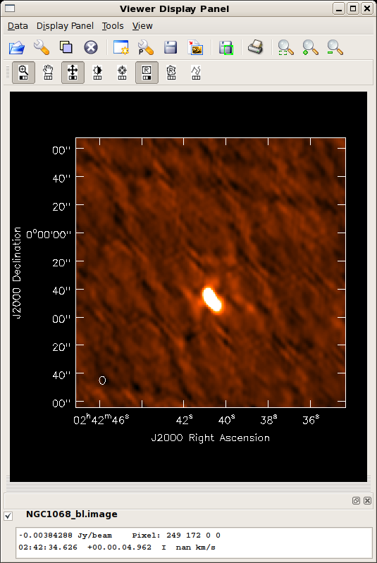
Initial clean image of NGC1068 *without* blcal.

Initial clean image of NGC1068 *with* blcal applied.

Although it makes only modest improvements for the present example, observations including a mix of EVLA and VLA telescopes may benefit from performing baseline-based corrections on a strong calibrator. Now that we have initial antenna-based solutions, we can use blcal.

default('blcal')
vis = 'ag733.ms'
# output baseline-based calibration solutions
caltable = 'cal.BL' 
# use the strong flux calibrator to determine baseline-based solutions
field = '0137+331' 
# generate a solution for each calibrator scan
solint = 'inf' 
gaintable = 'multisource.gcal'
 # calibration table with the best antenna-based solutions, so far
gainfield = '0137+331' 
# calibrator for the BL calibrator; in this example, gain cal and bl cal are the same
interp = 'nearest'
gaincurve = False
# do the first day's data
timerange = '2006/12/09/0:0:0~24:0:0'
blcal()
# now the second day
timerange = '2006/12/13/0:0:0~24:0:0'
blcal()

This operation generates the calibration table cal.BL. Solutions can be inspected with plotcal. Now we have to use applycal again to apply both the antenna-based and baseline-based calibration solutions to the data.

applycal(vis='ag733.ms', gaintable=['multisource.gcal', 'cal.BL'],
         gaincurve=False)

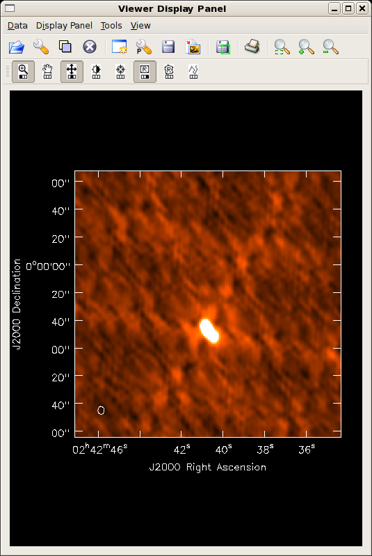
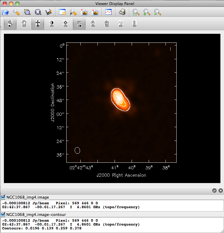
Did the blcal operation make a difference here? Getting ahead of ourselves a little, the plots at right show the initial clean images of NGC1068, one with blcal applied, and one without, and both images are displayed with the same stretch. There does appear a slight reduction of artifacts with blcal applied, but of course your mileage will vary.

Splitting the calibrated source data from the multisource measurement set

To split the calibrated source data out of the measurement set, use the CASA task split.

splitfile = 'NGC1667.split.ms'
rmtables(splitfile) # get rid of any old versions before splitting
split(vis='ag733.ms',outputvis=splitfile, datacolumn='corrected', field='NGC1667')

Alternatively, you can take advantage of scripting to loop over the sources.

for source in sourcelist:
    splitfile = source + '.split.ms'
    rmtables(splitfile)
    split(vis='ag733.ms',outputvis=splitfile, 
          datacolumn='corrected', field=source)

Imaging

An example desktop display of *viewer,* showing the image display panel, the data display options window, and the data loader.

Use clean for imaging and clean deconvolution. Like IMAGR in AIPS, it's worth some time mulling over all of the options. A complete list of keywords is given in the example, below. Most of the options should be relatively familiar to the AIPS user, but one keyword bears mentioning in this example: calready = True. By selecting this option, the CLEAN model is transformed back to (u,v) space and stored as as a new column in the visibility data. The transformed CLEAN model will be necessary for self calibration, described below.

For this snapshot survey, the example chooses a fairly conservative, slow clean to accommodate the less-than-ideal beam. You could probably get away with more efficient cleaning, but it's better to play it safe in scripted self-calibration.

default(clean)
mode                =      'mfs'        
niter               =       2000      
gain                =        0.1       
threshold           = '4.5e-5Jy'      
psfmode             =    'clark'       
imagermode          =  'csclean'     
cyclefactor    =          3       
cyclespeedup   =         -1       
multiscale          =         []       
interactive         =      False      
mask                =         []       
imsize              = [1024, 1024]      
cell                = ['0.75arcsec', '0.75arcsec']
stokes              =        'I'        
weighting           =  'natural'        
uvtaper             =      False      
pbcor               =      False      
minpb               =        0.1      
calready            =      True       
async               =      False      
for source in sourcelist:
    splitfile = source + '.split.ms'
    vis = splitfile
    imagename = source + '_img'
    rmtables(imagename + '*') # get rid of earlier versions of the image
    clean()

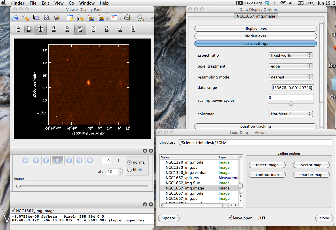
Take a look at the image using viewer.

viewer()

From the GUI, select the .image file you want to view, select Raster Image, and then dismiss and close your way through to the display.

Self-calibration

At this point we have a set of calibrated visibilities (the "splits") and a set of images. There's not much more that can be done for the fainter sources, but the brighter sources will almost certainly show some residual calibration artifacts that can be cleaned up with self-calibration. The strategy is to repeat using the primary calibration application gaincal, only this time we use the source itself as a calibrator.

NGC 1068 is a good example of a difficult source. Firstly, it's very bright, so residual phase calibration errors should be obvious. Secondly, like the larger fraction of the sky, it's located painfully close to the celestial equator, meaning that the (u,v) coverage is particularly poor.

To view the calibration artifacts, use viewer to display the image of NGC 1068, but adjust the display levels so that the displayed image saturates at 10 mJy. To do this, select the leftmost button bearing a wrench icon. The "Data Display Options" GUI opens, and you can enter the desired display stretch in the Data Range text box. To cutoff the stretch at 10 mJy,

Data Range: [-0.005,0.01]

You can see some residual systematics in the background and sidelobe artifacts that suggest the phase calibration isn't as good as it might be.

The process of self-calibration will involve iterating between (i) improved CLEAN models of the source (which are updated in the "split" visibility file so long as calready = True) and (i+1) improved calibrations generated by gaincal. For simplicity, in this example we will repeatedly generate new calibration tables so that we can avoid using accum.

Step i

In principle, we could start with the initial CLEAN model that we generated above. For this example, we'll take a more cautious approach and re-run clean interactively.

source = 'NGC1068' # set up a global variable to store the source we're working on
tget clean
vis = source + '.split.ms'
imagename = source + '_img0'
calready = True # make sure we store the model in the measurement set
interactive = True
go

The trick to interactive cleaning is to draw clean boxes around the sources as they appear in the residual image. By default, clean boxes are set by right-clicking on the image and dragging. The box can be edited until you double right-click inside the box, which then sets that box for cleaning. Press the green icon to continue cleaning the image; on the next major cycle, a new residual map will be displayed, affording the option to add clean boxes as new sources appear where they were once swamped by sidelobes.

Of course, for self-calibration, it pays to stop the cleaning early when artifacts start to appear in the residuals!

Step i + 1

To start, we should already have a clean model for NGC 1068 stored in the visibility database. Now we can set up gaincal.

default('gaincal') # reset inputs for gaincal (akin to RESTORE in AIPS)
vis = source + '.split.ms'
caltable = source + '.gcal0'
gaintype = 'G'
calmode = 'p' # phase-only self-calibration at this stage
solint = '10 min' # set up a fairly coarse correction interval in this early stage
minsnr = 3.0
gaintable = ''
field = source
gainfield = source # are these necessary?
gaincurve = False
gaincal() # or go!

Pause for Reflection and Troubleshooting

Self-calibration is a method to fine-tune your original calibration, and, as such, should produce relatively small phase corrections assuming the primary calibration was applied correctly. Now is a good time to run plotcal on your new calibration table (NGC1068.gcal0) to make sure the phase corrections range from a few to perhaps 10 or 20 degrees. If you see phase corrections greatly exceeding 20 degrees, then there's a chance of either

the primary calibration wasn't applied to the split database correctly, and should be checked, or
the model wasn't updated in the last iteration of clean, meaning you should verify that calready = True.

Step i + 2

Assuming plotcal gave reasonable results, next apply the calibration.

default('applycal')
vis = source + '.split.ms'
gaintable = source + '.gcal0'
gainfield = source
go

And now we can generate a new CLEAN model.

tget clean
imagename=source + '_img1' # choose an image root name that matches the future cal table to facilitate bookkeeping
go

Further Steps

Assuming things are going well, we can now continue to repeat the process until we are satisfied with the image.

Final, self-calibrated image of NGC1068.

tget gaincal
caltable = source +'.gcal1'
solint = "5 min" # halve the solution interval. 
go

# good idea to plotcal() again here!

tget applycal
gaintable = source + '.gcal1'
go

tget clean
imagename = source + '_img2'
go

And so on, decreasing the solution interval as much as the S/N and sampling allow.

Note that gaincal always uses the 'data' column (not the recently self-calibrated 'corrected' column) to find gain solutions. Therefore, these iterations simply serve to improve the data model, and gain solutions at each iteration are independent (e.g., the solution from the second self calibration iteration does not accumulate on top of the solution from the first interval. Use the CASA task accum if you wish to accumulate gain solutions).

One Last Iteration: Amplitude & Phase Self Calibration

After you have improved the phase calibration as much as possible, one last iteration where both phase and amplitude are calibrated can be beneficial. A&P self calibration should be performed with long solution intervals---typically the length of a scan.

default('gaincal') # reset inputs for gaincal (akin to RESTORE in AIPS)
vis = source + '.split.ms'
caltable = source + '.gcalap'
gaintype = 'G'
calmode = 'ap' # it's finally time to calibrate amplitudes, too
solint = 'inf' # one solution interval per scan (in conjunction with combine='') 
combine = ''
minsnr = 3.0
gaintable = source + '.gcal1' # apply your best phase calibration on the fly. 
gaincal() # or go!

Here, we are applying the best phase calibration solution on the fly by setting the gaintable parameter, so that this A&P self calibration iteration will only make small tweaks on top of the phase solutions we just worked so hard to find. Check your solutions in plotcal---amplitudes should not vary wildly and should be close to unity. If the solutions look reasonable, go ahead and apply the calibration:

default('applycal')
vis = source + '.split.ms'
gaintable = [source + '.gcal1', source + '.gcalap']
gainfield = source
go

The critical difference here from phase-only self calibration iterations is that we are applying two gain tables---the best phase solutions (source + '.gcal1') and the A&P solutions (source + '.gcalap'). Now you should be ready for one final imaging run with clean!

Last checked on CASA Version 3.0.0 (r9860).