Imaging a Mosaicked Spectral Line Dataset
As before, these notes assume that you have made the following global definitions in CASA:
# In CASA
msdir='./'
project='c0xxx'
msfile=msdir+project+'.ms'
and add one more (see the Special Note below):
# In CASA
mssplitfile=msdir+project_'split.ms'
If your data are already edited and calibrated, there's really only one step left: clean. Unlike in MIRIAD, which has separate tasks for inverting and cleaning an image, CASA does it in one step. If you want a dirty image, just set niter=0 so that clean doesn't actually do any...cleaning.
Beta-alert: As of the 3.0.0 release, a bug in one of the routines which assembles data (likely concat) may create problems if your dataset contains spectral windows with differing numbers of channels, e.g. if you have a wideband mode with a smaller number of broad channels to calibrate your narrowband windows with lots of channels. The recognizable symptom is an immediate, severe "table conformance error" that returns you to the CASA command line. Making an MS containing only the narrowband channels (presumably, each having the same number) using split will solve this problem.
For the specific example of an MS containing one wideband window (spw 0) followed by two narrowband windows (spw 1,2), here's how to split off the narrowband windows into their own MS:
# In CASA
split(vis=msfile,spw='1~2',field='',outputvis=mssplitfile)
We use this output file (mssplitfile), which now contains only the narrowband windows as spw 0 and 1, in the clean command example below; if your dataset contains only windows with the same number of channels you may use your original msfile (with an appropriate choice of spw, of course).
Here's a command-line call to clean, which demonstrates many of the interesting parameters you can tweak. This is a simple example, assuming you are making an image of the entire mosaic, and you want to clean the whole thing.
Some things of note (input parameters are italicized):
- phasecenter doesn't need to be specified, if you are happy with the phase center at the position of the first of the observed source fields.
- it is important for both imagermode and ftmachine to be set to 'mosaic' if you want your mosaicked data to be stitched together correctly (this should happen by default).
- the parameters pbcor and minpb set whether or not a primary beam correction is done, and how far out, respectively.
- always include units when specifying the threshold at which to stop cleaning.
# In CASA
clean(vis=mssplitfile,imagename='clean_pb',spw='0~1',field='3~51',
      phasecenter='J2000 20h35m35.32 60d10m01.00',
      cell=2.,imsize=[400,400],
      mode='velocity',start='-103.00km/s',width='5.08km/s',nchan=29,
      interpolation='linear',psfmode='clark',
      imagermode='mosaic',ftmachine='mosaic',
      scaletype='SAULT',restfreq='115.2712GHz',interactive=F,
      minpb=0.1,pbcor=True,
      niter=1000,threshold='340mJy',mosweight=False,
      weighting='natural')
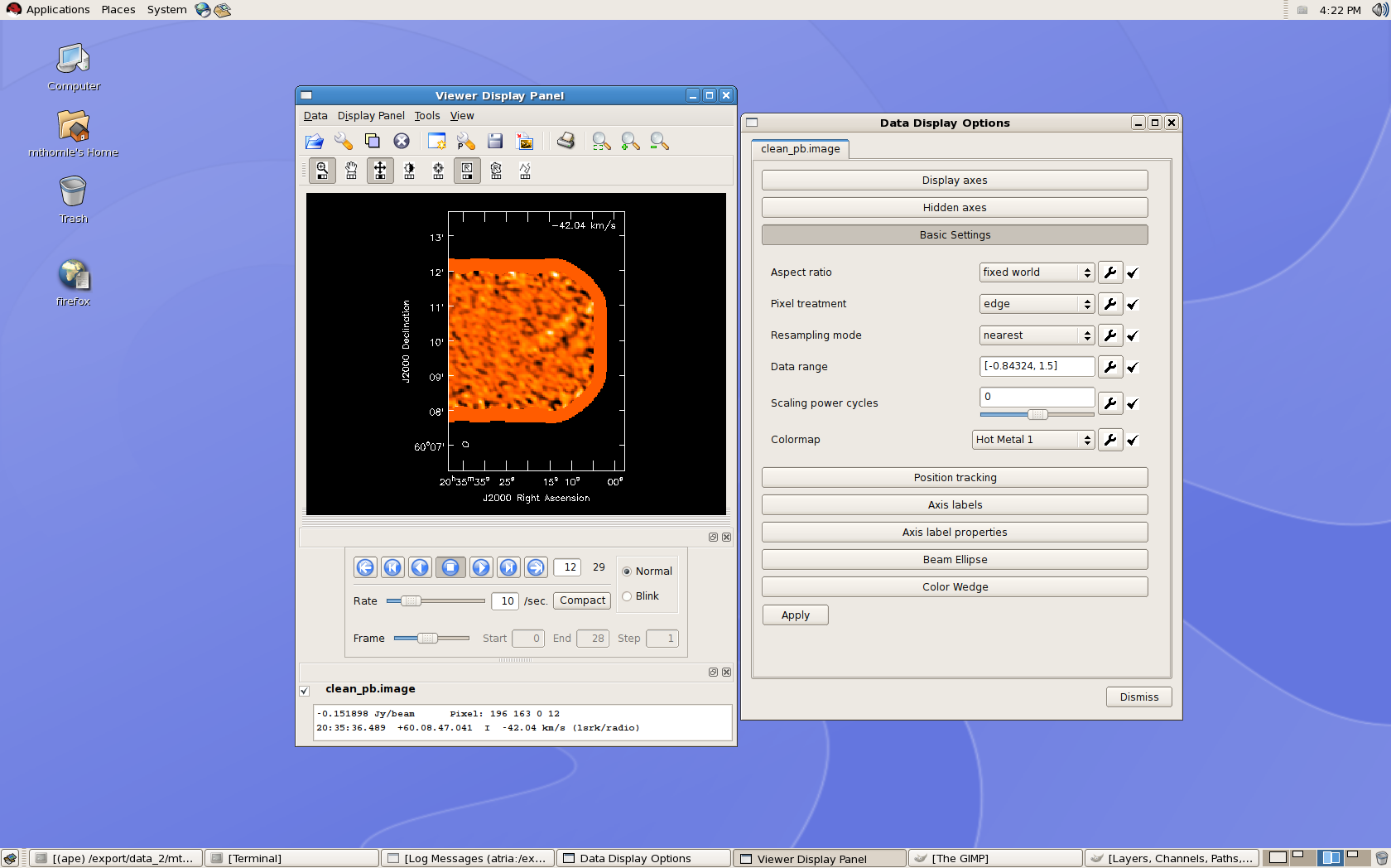
To take a look at the image you produced, use the CASA viewer:
# In CASA
viewer(infile='clean_pb.image')

The lower part of the Viewer Display Panel provides buttons which allow you to navigate between spectral channels, and the coordinate and flux information of the pixel under the cursor is displayed at the bottom of this window. The Data Display Options window allows you to adjust the data range for the color scale as well as a number of plotting options (e.g., whether information about the third dimension of the cube is displayed in the upper right corner.)