EVLA Wide-Band Wide-Field Imaging: G55.7 - CASA4.2
- This CASA Guide is designed for CASA v4.1. If you are using an older version of CASA please see the same guide for CASA v4.1, CASA v4.0, or CASA v3.4.
EVLA Wide-Band Wide-Field Imaging: G55.7 - CASA4.2
Overview
This CASA Guide describes the imaging of the supernova remnant G55.7+3.4.. The data were taken on August 23, 2010, in the first D-configuration for which the new wide-band capabilities of the WIDAR correlator were available. The 8-hour-long observation includes all available 1 GHz of bandwidth in L-band, from 1-2 GHz in frequency.
Obtaining the data
A copy of the data can be downloaded here: http://casa.nrao.edu/Data/EVLA/G55/G55.7+3.4_10s.ms.tar.gz
Note that this dataset is rather large: ~15GB
As a start, unzip and untar the data:
tar -xzvf G55.7+3.4_10s.ms.tar.gz
This will take a minute, but once it's complete, you will have a directory called G55.7+3.4_10s.ms which is the data. Online flags have been applied (which delete known bad data), some uninteresting scans removed, and the data time-averaged to 10 seconds. (The data were taken in D-configuration, where maximum baselines are 1 km, so one can safely average to 3s or even 10s to reduce data set size.) This is equivalent to what you would download from the archive if you requested time-averaging, scans 16~313, and application of the online flags.
You can also find the dataset in the NRAO archive. Note that it is 170 GB in raw form.
Averaging to 10 seconds and the removal of some scans which are not used in this tutorial reduces the size of the data set to around 15 GB; the addition of columns for model and corrected data (known as "scratch columns") during calibration will ultimately inflate the MS by a factor of a few in size (to around 45 GB).
Start and confirm your version of CASA
Start CASA by typing casapy on the command line. If you have not used CASA before, some helpful tips are available on the Getting Started in CASA page.
This guide has been written for CASA release 4.2.0. Please confirm your version before proceeding.
# In CASA
version = casalog.version()
print "You are using " + version
if (int(version.split()[4][1:-1]) < 28322):
    print "\033[91m YOUR VERSION OF CASA IS TOO OLD FOR THIS GUIDE."
    print "\033[91m PLEASE UPDATE IT BEFORE PROCEEDING."
else:
    print "Your version of CASA is appropriate for this guide."
Preliminary data evaluation
As a first step, use listobs to have a look at the MS:
# In CASA
listobs('G55.7+3.4_10s.ms')
Note that throughout this tutorial, we will run tasks using the task(parameter=value) syntax. When called in this manner, all parameters not explicitly set will use their default values.
The logger output will look like this:
##########################################
##### Begin Task: listobs            #####
listobs(vis="G55.7+3.4_10s.ms",selectdata=True,spw="",field="",
        antenna="",uvrange="",timerange="",correlation="",scan="",
        intent="",feed="",array="",observation="",verbose=True,
        listfile="")
================================================================================
           MeasurementSet Name:  /scr2/casa/evla_G55/G55.7+3.4_10s.ms      MS Version 2
================================================================================
   Observer: Dr. Sanjay Sanjay Bhatnagar     Project: T.B.D.
Observation: EVLA
Data records: 7343848       Total integration time = 26691.5 seconds
   Observed from   23-Aug-2010/01:00:25.0   to   23-Aug-2010/08:25:16.5 (UTC)

   ObservationID = 0         ArrayID = 0
  Date        Timerange (UTC)          Scan  FldId FieldName           nRows   Int(s)   SpwIds      ScanIntent
  23-Aug-2010/01:00:25.0 - 01:01:00.5    16      1 J1925+2106          8008   7.79     [0, 1, 2, 3, 4, 5, 6, 7]    CALIBRATE_PHASE.UNSPECIFIED
              01:01:10.0 - 01:02:30.0    17      1 J1925+2106          25272  10       [0, 1, 2, 3, 4, 5, 6, 7]    CALIBRATE_PHASE.UNSPECIFIED
              01:02:40.0 - 01:04:00.0    18      1 J1925+2106          25272  10       [0, 1, 2, 3, 4, 5, 6, 7]    CALIBRATE_PHASE.UNSPECIFIED
              01:04:10.0 - 01:05:29.5    19      1 J1925+2106          25272  9.89     [0, 1, 2, 3, 4, 5, 6, 7]    CALIBRATE_PHASE.UNSPECIFIED
              01:05:39.0 - 01:06:59.0    20      1 J1925+2106          25272  9.89     [0, 1, 2, 3, 4, 5, 6, 7]    CALIBRATE_PHASE.UNSPECIFIED
              01:07:12.0 - 01:08:29.0    21      2 G55.7+3.4           25064  9.33     [0, 1, 2, 3, 4, 5, 6, 7]    OBSERVE_TARGET.UNSPECIFIED
              01:08:39.0 - 01:09:59.0    22      2 G55.7+3.4           25272  10       [0, 1, 2, 3, 4, 5, 6, 7]    OBSERVE_TARGET.UNSPECIFIED
              01:10:09.0 - 01:11:29.0    23      2 G55.7+3.4           25272  10       [0, 1, 2, 3, 4, 5, 6, 7]    OBSERVE_TARGET.UNSPECIFIED
              01:11:39.0 - 01:12:58.5    24      2 G55.7+3.4           25272  9.89     [0, 1, 2, 3, 4, 5, 6, 7]    OBSERVE_TARGET.UNSPECIFIED
              01:13:08.0 - 01:14:28.0    25      2 G55.7+3.4           25272  10       [0, 1, 2, 3, 4, 5, 6, 7]    OBSERVE_TARGET.UNSPECIFIED
              01:14:38.0 - 01:15:58.0    26      2 G55.7+3.4           25272  10       [0, 1, 2, 3, 4, 5, 6, 7]    OBSERVE_TARGET.UNSPECIFIED
              01:16:08.0 - 01:17:28.0    27      2 G55.7+3.4           25272  10       [0, 1, 2, 3, 4, 5, 6, 7]    OBSERVE_TARGET.UNSPECIFIED
              01:17:38.0 - 01:18:57.5    28      2 G55.7+3.4           25272  9.89     [0, 1, 2, 3, 4, 5, 6, 7]    OBSERVE_TARGET.UNSPECIFIED
              01:19:07.0 - 01:20:27.0    29      2 G55.7+3.4           25272  10       [0, 1, 2, 3, 4, 5, 6, 7]    OBSERVE_TARGET.UNSPECIFIED
              01:20:37.0 - 01:21:57.0    30      2 G55.7+3.4           25272  10       [0, 1, 2, 3, 4, 5, 6, 7]    OBSERVE_TARGET.UNSPECIFIED
<snip>
              08:04:31.0 - 08:05:50.5   300      2 G55.7+3.4           25272  9.89     [0, 1, 2, 3, 4, 5, 6, 7]    OBSERVE_TARGET.UNSPECIFIED
              08:06:00.0 - 08:07:20.0   301      2 G55.7+3.4           25272  10       [0, 1, 2, 3, 4, 5, 6, 7]    OBSERVE_TARGET.UNSPECIFIED
              08:07:30.0 - 08:08:50.0   302      2 G55.7+3.4           25272  10       [0, 1, 2, 3, 4, 5, 6, 7]    OBSERVE_TARGET.UNSPECIFIED
              08:09:00.0 - 08:10:20.0   303      2 G55.7+3.4           25272  10       [0, 1, 2, 3, 4, 5, 6, 7]    OBSERVE_TARGET.UNSPECIFIED
              08:10:30.0 - 08:11:49.5   304      2 G55.7+3.4           25272  9.89     [0, 1, 2, 3, 4, 5, 6, 7]    OBSERVE_TARGET.UNSPECIFIED
              08:11:59.0 - 08:13:19.0   305      2 G55.7+3.4           25272  10       [0, 1, 2, 3, 4, 5, 6, 7]    OBSERVE_TARGET.UNSPECIFIED
              08:13:29.0 - 08:14:48.5   306      2 G55.7+3.4           25272  9.89     [0, 1, 2, 3, 4, 5, 6, 7]    OBSERVE_TARGET.UNSPECIFIED
              08:17:50.5 - 08:17:50.5   308      3 0542+498=3C147      80     4        [0, 1, 2, 3, 4, 5, 6, 7]    CALIBRATE_AMPLI.UNSPECIFIED,UNSPECIFIED.UNSPECIFIED,CALIBRATE_BANDPASS.UNSPECIFIED
              08:17:59.0 - 08:19:18.5   309      3 0542+498=3C147      17152  9.36     [0, 1, 2, 3, 4, 5, 6, 7]    CALIBRATE_AMPLI.UNSPECIFIED,UNSPECIFIED.UNSPECIFIED,CALIBRATE_BANDPASS.UNSPECIFIED
              08:19:28.0 - 08:20:48.0   310      3 0542+498=3C147      18216  10       [0, 1, 2, 3, 4, 5, 6, 7]    CALIBRATE_AMPLI.UNSPECIFIED,UNSPECIFIED.UNSPECIFIED,CALIBRATE_BANDPASS.UNSPECIFIED
              08:20:58.0 - 08:22:18.0   311      3 0542+498=3C147      18216  10       [0, 1, 2, 3, 4, 5, 6, 7]    CALIBRATE_AMPLI.UNSPECIFIED,UNSPECIFIED.UNSPECIFIED,CALIBRATE_BANDPASS.UNSPECIFIED
              08:22:28.0 - 08:23:47.5   312      3 0542+498=3C147      18216  9.89     [0, 1, 2, 3, 4, 5, 6, 7]    CALIBRATE_AMPLI.UNSPECIFIED,UNSPECIFIED.UNSPECIFIED,CALIBRATE_BANDPASS.UNSPECIFIED
              08:23:57.0 - 08:25:16.5   313      3 0542+498=3C147      18216  9.89     [0, 1, 2, 3, 4, 5, 6, 7]    CALIBRATE_AMPLI.UNSPECIFIED,UNSPECIFIED.UNSPECIFIED,CALIBRATE_BANDPASS.UNSPECIFIED
           (nRows = Total number of rows per scan)
Fields: 3
  ID   Code Name                RA              Decl          Epoch   SrcId nRows
  1    D    J1925+2106          19:25:59.60537 +21.06.26.1622 J2000   1     1004816
  2    NONE G55.7+3.4           19:21:40.00000 +21.45.00.0000 J2000   2     6248936
  3    N    0542+498=3C147      05:42:36.13792 +49.51.07.2336 J2000   3     90096
   (nVis = Total number of time/baseline visibilities per field)
Spectral Windows:  (8 unique spectral windows and 1 unique polarization setups)
  SpwID  #Chans Frame Ch1(MHz)    ChanWid(kHz)  TotBW(kHz)  Corrs
  0          64 TOPO  1000        2000          128000      RR  RL  LR  LL
  1          64 TOPO  1128        2000          128000      RR  RL  LR  LL
  2          64 TOPO  1256        2000          128000      RR  RL  LR  LL
  3          64 TOPO  1384        2000          128000      RR  RL  LR  LL
  4          64 TOPO  1520        2000          128000      RR  RL  LR  LL
  5          64 TOPO  1648        2000          128000      RR  RL  LR  LL
  6          64 TOPO  1776        2000          128000      RR  RL  LR  LL
  7          64 TOPO  1904        2000          128000      RR  RL  LR  LL
Sources: 24
  ID   Name                SpwId RestFreq(MHz)  SysVel(km/s)
  1    J1925+2106          0     -              -
  1    J1925+2106          1     -              -
  1    J1925+2106          2     -              -
  1    J1925+2106          3     -              -
  1    J1925+2106          4     -              -
  1    J1925+2106          5     -              -
  1    J1925+2106          6     -              -
  1    J1925+2106          7     -              -
  2    G55.7+3.4           0     -              -
  2    G55.7+3.4           1     -              -
  2    G55.7+3.4           2     -              -
  2    G55.7+3.4           3     -              -
  2    G55.7+3.4           4     -              -
  2    G55.7+3.4           5     -              -
  2    G55.7+3.4           6     -              -
  2    G55.7+3.4           7     -              -
  3    0542+498=3C147      0     -              -
  3    0542+498=3C147      1     -              -
  3    0542+498=3C147      2     -              -
  3    0542+498=3C147      3     -              -
  3    0542+498=3C147      4     -              -
  3    0542+498=3C147      5     -              -
  3    0542+498=3C147      6     -              -
  3    0542+498=3C147      7     -              -
Antennas: 27:
  ID   Name  Station   Diam.    Long.         Lat.
  0    ea01  W09       25.0 m   -107.37.25.2  +33.53.51.0
  1    ea02  E02       25.0 m   -107.37.04.4  +33.54.01.1
  2    ea03  E09       25.0 m   -107.36.45.1  +33.53.53.6
  3    ea04  W01       25.0 m   -107.37.05.9  +33.54.00.5
  4    ea05  W08       25.0 m   -107.37.21.6  +33.53.53.0
  5    ea06  N06       25.0 m   -107.37.06.9  +33.54.10.3
  6    ea07  E05       25.0 m   -107.36.58.4  +33.53.58.8
  7    ea08  N01       25.0 m   -107.37.06.0  +33.54.01.8
  8    ea09  E06       25.0 m   -107.36.55.6  +33.53.57.7
  9    ea10  N03       25.0 m   -107.37.06.3  +33.54.04.8
  10   ea11  E04       25.0 m   -107.37.00.8  +33.53.59.7
  11   ea12  E08       25.0 m   -107.36.48.9  +33.53.55.1
  12   ea13  N07       25.0 m   -107.37.07.2  +33.54.12.9
  13   ea15  W06       25.0 m   -107.37.15.6  +33.53.56.4
  14   ea16  W02       25.0 m   -107.37.07.5  +33.54.00.9
  15   ea17  W07       25.0 m   -107.37.18.4  +33.53.54.8
  16   ea18  N09       25.0 m   -107.37.07.8  +33.54.19.0
  17   ea19  W04       25.0 m   -107.37.10.8  +33.53.59.1
  18   ea20  N05       25.0 m   -107.37.06.7  +33.54.08.0
  19   ea21  E01       25.0 m   -107.37.05.7  +33.53.59.2
  20   ea22  N04       25.0 m   -107.37.06.5  +33.54.06.1
  21   ea23  E07       25.0 m   -107.36.52.4  +33.53.56.5
  22   ea24  W05       25.0 m   -107.37.13.0  +33.53.57.8
  23   ea25  N02       25.0 m   -107.37.06.2  +33.54.03.5
  24   ea26  W03       25.0 m   -107.37.08.9  +33.54.00.1
  25   ea27  E03       25.0 m   -107.37.02.8  +33.54.00.5
  26   ea28  N08       25.0 m   -107.37.07.5  +33.54.15.8

##### End Task: listobs              #####
##########################################
We can see that there are three sources in this observation:
- J1925+2106, field ID 1: the phase calibrator;
- G55.7+3.4, field ID 2: the supernova remnant;
- 0542+498=3C147, field ID 3: the flux and bandpass calibrator.
We can also see that these sources have associated "scan intents", which indicate their function in the observation. Note that you can select sources based on their intents in certain CASA tasks. The various scan intents in this dataset are:
- CALIBRATE_PHASE indicates that this is a scan to be used for gain calibration;
- OBSERVE_TARGET indicates that this is the science target;
- CALIBRATE_AMPLI indicates that this is to be used for flux calibration; and
- CALIBRATE_BANDPASS indicates that these scans are to be used for bandpass calibration.
Note that 3C147 is to be used for both flux and bandpass calibration.
We can see the antenna configuration for this observation using plotants:
# In CASA
plotants('G55.7+3.4_10s.ms')
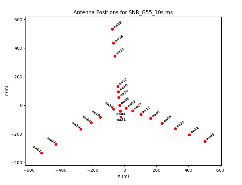
This shows that antennas ea01, ea18, and ea03 were on the extreme ends of the west, north, and east arms, respectively. The antenna position diagram is particularly useful as a guide to help determine which antenna to use as the reference antenna later during calibration.
We may also inspect the raw data using plotms. To start with, let's look at a subset of scans on the supernova remnant:
# In CASA
plotms(vis='G55.7+3.4_10s.ms', scan='30,75,120,165,190,235,303',
       antenna='ea24', xaxis='freq', yaxis='amp', coloraxis='spw',
       iteraxis='scan', correlation='RR,LL', symbolshape='circle')
The coloraxis parameter indicates that a different color will be assigned to each spectral window, and the iteraxis parameter tells plotms to display a new plot for each scan. We have chosen only one antenna (ea24) and just the right and left circular polarizations (without the cross-hand terms) to reduce the amount of data in the selection. One can flip through these plots using the green arrows located at the bottom of the plotting GUI: the double-left arrow will display the very first plot in the set, the single left arrow will go back one plot, and the right arrows have similar behavior for moving forward in the set.
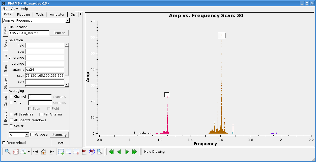
Flipping through the scans, it's clear that there is significant time- and frequency-variable RFI present in this observation. Since this is L-band data taken in the most compact EVLA configuration ("D"), this comes as no surprise. However, it also poses one of the greatest challenges for obtaining a good image.
In particular, we can see that two spectral windows (SPWs) are quite badly affected. To determine which these are, click in the "Mark Regions" tool at the bottom of the plotms GUI (the open box with a green "plus" sign), and use the mouse to select a few of the highest-amplitude points in each of these SPWs. Click on the "Locate" button (magnifying glass sign), and information associated with the selected points will be displayed in the logger window:
Frequency in [1.22177 1.27139] or [1.5762 1.65063], Amp in [23.1713 24.3056] or [59.6296 63.6806]:
Scan=30 Field=G55.7+3.4[2] Time=2010/08/23/01:20:57.0 BL=ea12@E08 & ea24@W05[11&22] Spw=1 Chan=59 Freq=1.246 Corr=RR X=1.246 Y=23.5243  (38134/11/1526)
Scan=30 Field=G55.7+3.4[2] Time=2010/08/23/01:21:07.0 BL=ea03@E09 & ea24@W05[2&22] Spw=1 Chan=59 Freq=1.246 Corr=RR X=1.246 Y=23.6116  (40310/12/374)
Scan=30 Field=G55.7+3.4[2] Time=2010/08/23/01:21:07.0 BL=ea12@E08 & ea24@W05[11&22] Spw=1 Chan=59 Freq=1.246 Corr=RR X=1.246 Y=23.4432  (41462/12/1526)
Scan=30 Field=G55.7+3.4[2] Time=2010/08/23/01:21:57.0 BL=ea03@E09 & ea24@W05[2&22] Spw=1 Chan=59 Freq=1.246 Corr=RR X=1.246 Y=23.7536  (56950/17/374)
Scan=30 Field=G55.7+3.4[2] Time=2010/08/23/01:21:07.0 BL=ea12@E08 & ea24@W05[11&22] Spw=4 Chan=41 Freq=1.602 Corr=RR X=1.602 Y=61.9097  (131282/39/1490)
Scan=30 Field=G55.7+3.4[2] Time=2010/08/23/01:21:17.0 BL=ea12@E08 & ea24@W05[11&22] Spw=4 Chan=41 Freq=1.602 Corr=RR X=1.602 Y=61.1769  (134610/40/1490)
Scan=30 Field=G55.7+3.4[2] Time=2010/08/23/01:21:27.0 BL=ea12@E08 & ea24@W05[11&22] Spw=4 Chan=41 Freq=1.602 Corr=RR X=1.602 Y=60.1834  (137938/41/1490)
Found 7 points (7 unflagged) among 239616 in 0.02s.
We can see that SPWs 1 and 4 are among the worst affected by RFI. (As an aside, note that the syntax for reporting a selected point's baseline is {antenna 1 name}@{pad 1 name} &{antenna 2 name}@{pad 2 name}[{antenna 1 index}&{antenna 2 index}].) At this point, feel free to play around a bit more with plotms; you might try experimenting with different axes for iteration (under the "Iter" left-hand tab), different data selection parameters (under "Data"), different axes ("Axes"), different averaging techniques (under "Data"), or different selections for the coloraxis (the "colorize" option under "Display").
A priori calibration and flagging
Before we proceed with further processing, we should check the observation log to see if there were any issues noted during the run that need to be addressed. The observing log file is linked to the archive web page for this observation (at far right; under "logs etc."). Looking at the log, we can see that antenna ea07 may need a position correction, and antennas ea06, ea17, ea20, and ea26 did not have L-band receivers installed at the time and should be flagged.
Antenna position correction
Correcting a known position error for an antenna is done with the task gencal. This is important, because the observed visibilities are a function of [math]\displaystyle{ u }[/math] and [math]\displaystyle{ v }[/math]. If an antenna's position is incorrect, then [math]\displaystyle{ u }[/math] and [math]\displaystyle{ v }[/math] will be calculated incorrectly, and there will be errors in any image derived from the data. Of course, the a priori position corrections may not completely account for all errors.
The gencal task will query the VLA Baseline Corrections database to determine what baseline corrections to apply to the dataset. If you wish to double-check this by hand, refer to the EVLA/VLA Baseline Corrections page.
# In CASA
gencal(vis='G55.7+3.4_10s.ms', caltable='G55.7+3.4_10s.pos',
       caltype='antpos')
As reported by the CASA logger, gencal found a position correction for antenna ea07 of (x, y, z) = (0.0087, 0.0137, 0.000) and recorded this in our specified calibration table.
Gain curve and opacity correction
A decision has been made here to ignore both the corrections for atmospheric opacity and for the elevation-dependent telescope gain throughout this tutorial. These effects are very small (less than or about 1%) across the frequency range of this observation (1-2 GHz). At higher frequencies, these corrections may be important and the appropriate calibration tables can be computed using the task gencal. For an example of a tutorial which corrects for atmospheric opacity and the elevation-dependent gain see this [tutorial.]
Flagging non-operational antennas
In addition to updating the position for antenna ea07, we have to flag antennas ea06, ea17, ea20, and ea26, since these did not have working L-band receivers at the time of observation. We do this with the task flagdata:
# In CASA
flagdata(vis='G55.7+3.4_10s.ms', mode='manual',
         antenna='ea06,ea17,ea20,ea26')
Note that the first thing flagdata does is create a backup flag file, in this case named "flagdata_1". This flag file contains a copy of the flags present in the MS prior to the requested flagging operation, and can be found inside the <MS_name>.flagversions directory, along with any other backed up flag files. Since these flag files take up a fair amount of space (in this particular case, 230 MB), we won't me making them every time we run flagdata -- the automatic flag backup can be turned off by setting flagbackup=False. However, it's good to keep a record of the names of the backup files and the associated processing step, in case you wish to restore a previous version of the flags using the flagmanager task.
Flagging shadowed antennas and zero-amplitude data
Since this is the most compact EVLA configuration, there may be instances where one antenna blocks, or "shadows" another. Therefore, we will run flagdata to remove these data:
# In CASA
flagdata(vis='G55.7+3.4_10s.ms', mode='shadow',
         flagbackup=False)
In this particular observation, there does not appear to be any data affected by shadowing, as can be seen in the logger report.
In addition, there may be times during which the correlator writes out pure zero-valued data. In order to remove this bad data, we run flagdata to remove any pure zeroes:
# In CASA
flagdata(vis='G55.7+3.4_10s.ms', mode='clip',
         clipzeros=True, flagbackup=False)
Inspecting the logger output which is generated by flagdata shows that there is a very small quantity of zero-valued data (0.02%) present in this MS.
Note that the archive will automatically flag shadowed antennas as well as zero-valued data, if you request that online flags are applied.
Automatic RFI excision
Now, we move on to one of the most difficult parts of L-band, D-configuration data processing: excising the RFI. For the original reduction of this MS, flagging was done by hand and took several weeks. The resulting data are offered as an option for the imaging stage of this tutorial (because careful by-hand flagging does yield a better image); however, it's not always practical to undertake this endeavor, and often the "automatic" flagging provides a reasonable (and much less time-consuming) solution. Therefore, we will demonstrate the use of the automatic RFI excision tools currently available in CASA.
Hanning-smoothing data
Prior to flagging any data which is affect by strong RFI, one should Hanning-smooth the data to remove Gibbs ringing. This is done with the task hanningsmooth, which can either write a new, Hanning-smoothed MS or directly operate on the requested column of the input MS. To conserve space, we will request the latter. Note that if you wish to make your own "before" and "after" plots, you should make the first prior to running hanningsmooth, since you will be overwriting the non-Hanning-smoothed data in the process -- and this is not reversible.
# In CASA
plotms(vis='G55.7+3.4_10s.ms', scan='30', antenna='ea24', spw='0~2',
    xaxis='freq', yaxis='amp', coloraxis='spw', symbolshape = 'circle',
    correlation='RR,LL', plotrange=[1.0,1.27,-0.3,2.5],
    plotfile='amp_v_freq.beforeHanning.png')

hanningsmooth(vis='G55.7+3.4_10s.ms', datacolumn='data')

plotms(vis='G55.7+3.4_10s.ms', scan='30', antenna='ea24', spw='0~3',
    xaxis='freq', yaxis='amp', coloraxis='spw', symbolshape = 'circle',
    correlation='RR,LL', plotrange=[1.0,1.27,-0.3,2.5],
    plotfile='amp_v_freq.afterHanning.png')
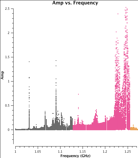
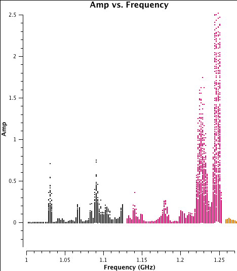
Task hanningsmooth will take a few minutes to run. Note that the 2nd plotms command above contains a trivial change in the spw selection (trivial because the 4th spw is outside of the specified plotrange). This forces plotms to reload the plot since by default, plotms will not redraw a plot if the input parameters are unchanged. In this case, since the data column was changed between calls to plotms, a redraw is necessary. When using the GUI, you can simply check "force reload" in the bottom left corner of the side bar before clicking "Plot."
We can compare the Hanning-smoothed data with the raw data by plotting a subset of data to show the result of Hanning-smoothing (see plots to the left and right). As you can see, the smoothing has spread the single-channel RFI into three channels, but has also removed the effects of some of the worst RFI from a number of channels. Overall, this will improve our ability to flag RFI from the data and retain as much good data as possible.
Using phase calibration source for preliminary bandpass calibration
In order to get the best possible result from the automatic RFI excision, we will first apply bandpass calibration to the MS. Since the RFI is time-variable, using the phase calibration source to make an average bandpass over the entire observation will mitigate the amount of RFI present in the calculated bandpass. (For the final calibration, we will use the designated bandpass source 3C147; however, since this object was only observed in the last set of scans, it doesn't sample the time variability and would not provide a good average bandpass.)
Since there are likely to be gain variations over the course of the observation, we will run gaincal to solve for an initial set of antenna-based phases over a narrow range of channels. These will be used to create the bandpass solutions. While amplitude variations will have little effect on the bandpass solutions, it is important to solve for these phase variations with sufficient time resolution to prevent decorrelation when vector averaging the data in computing the bandpass solutions.
In order to choose a narrow range of channels for each spectral window which are relatively RFI-free over the course of the observation, we can look at the data with plotms. Note that it's important to only solve for phase using a narrow channel range, since an antenna-specific delay will cause the phase to vary with respect to frequency over the spectral window, perhaps by a substantial amount.
# In CASA
plotms(vis='G55.7+3.4_10s.ms', scan='30,75,120,165,190,235,303',
       antenna='ea24', xaxis='channel', yaxis='amp', iteraxis='spw',
       yselfscale=True, correlation='rr,ll')
- yselfscale=True: sets the y-scaling to be for the currently displayed spectral window, since some spectral windows have much worse RFI and will skew the scale for others.
Looking at these plots, we can choose appropriate channel ranges for each SPW:
SPW 0: 10-13
SPW 1: 30-33
SPW 2: 32-35
SPW 3: 30-33
SPW 4: 35-38
SPW 5: 30-33
SPW 6: 30-33
SPW 7: 46-49
Using these channel ranges, we run gaincal to perform phase-only solutions over the course of the observation:
# In CASA
gaincal(vis='G55.7+3.4_10s.ms', caltable='G55.7+3.4_10s.initPh',
        intent='CALIBRATE_PHASE*', solint='int',
        spw='0:10~13,1;3;5~6:30~33,2:32~35,4:35~38,7:46~49',
        refant='ea24', minblperant=3,
        minsnr=3.0, calmode='p', gaintable='G55.7+3.4_10s.pos')
- caltable='G55.7+3.4_10s.initPh': this is the output calibration table that will be written.
- intent='CALIBRATE_PHASE*': this is the way we have chosen to select data. Alternatively, we could have used "field='J1925+2106'", since this is the only source with the CALIBRATE_PHASE* scan intent. Note the use of the wildcard character "*" at the end of the string; this accounts for the fact that all the intents end with ".UNSPECIFIED". We could just as well have used "*PHASE*".
- solint='int': we request a solution for each 10-second integration.
- spw='0:10~13,1;3;5~6:30~33,2:32~35,4:35~38,7:46~49': note the syntax of this selection: a ":" is used to separate the SPW from channel selection, ";" is used to separate within this selection, and "~" is used to indicate an inclusive range.
- refant='ea24': we have chosen ea24 as the reference antenna after inspecting the antenna position diagram (see above). It is relatively close to, but not directly in, the center of the array, which could be important in D-configuration, since you don't want the reference antenna to have a high probability of being shadowed by nearby antennas.
- minblperant=3: the minimum number of baselines which must be present to attempt a phase solution.
- minsnr=3.0: the minimum signal-to-noise a solution must have to be considered acceptable. Note that solutions which fail this test will cause these data to be flagged downstream of this calibration step.
- calmode='p': perform phase-only solutions.
- gaintable='G55.7+3.4_10s.pos': use the antenna position correction for ea07 that we created earlier.
Note that a number of solutions do not pass the requirements of the minimum 3 baselines (generating the terminal message "Insufficient unflagged antennas to proceed with this solve.") or minimum signal-to-noise ratio (outputting "n of x solutions rejected due to SNR < 3 ..."). A particularly large number of solutions are rejected in SPW 4, where the RFI is most severe.
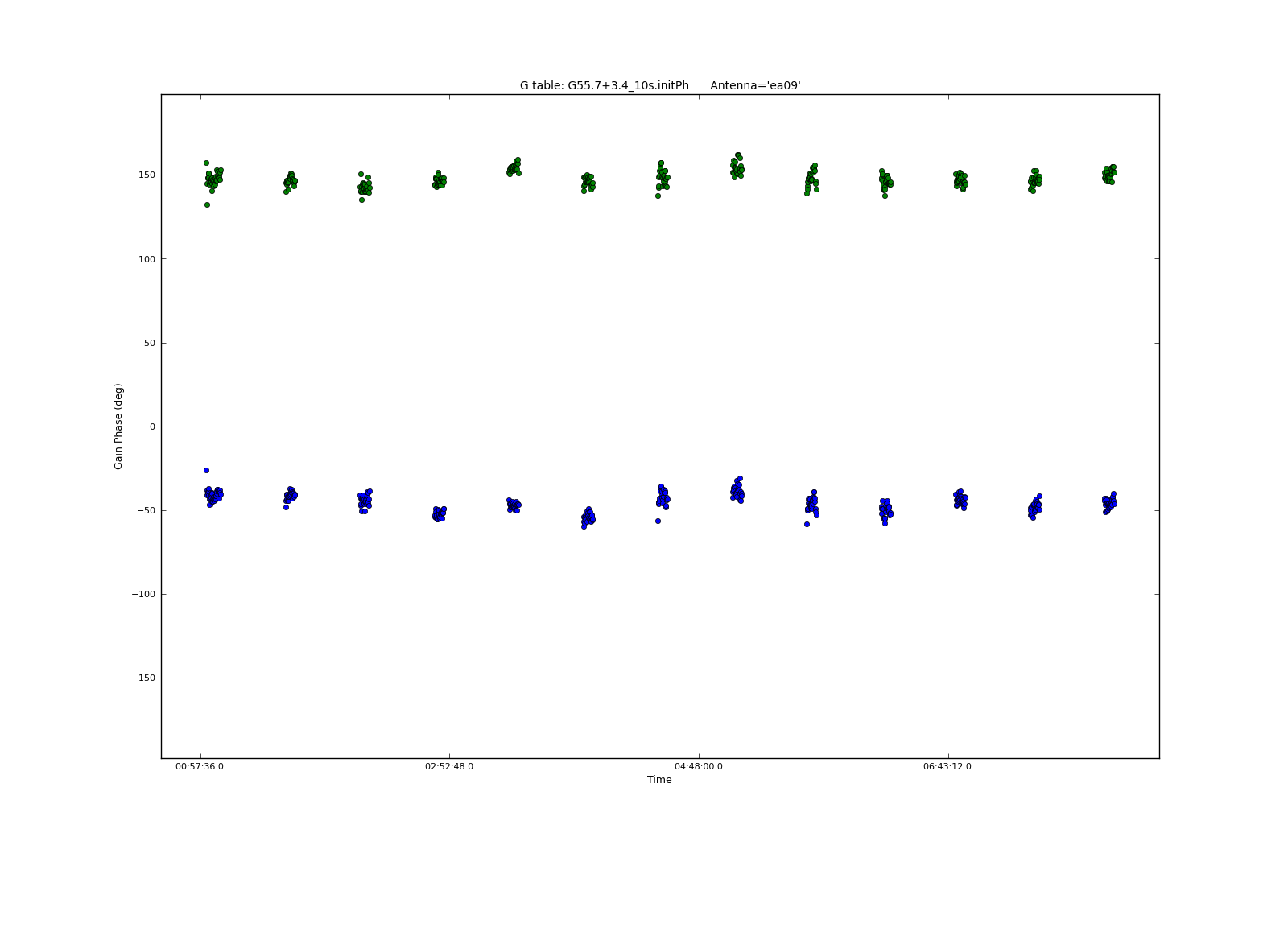
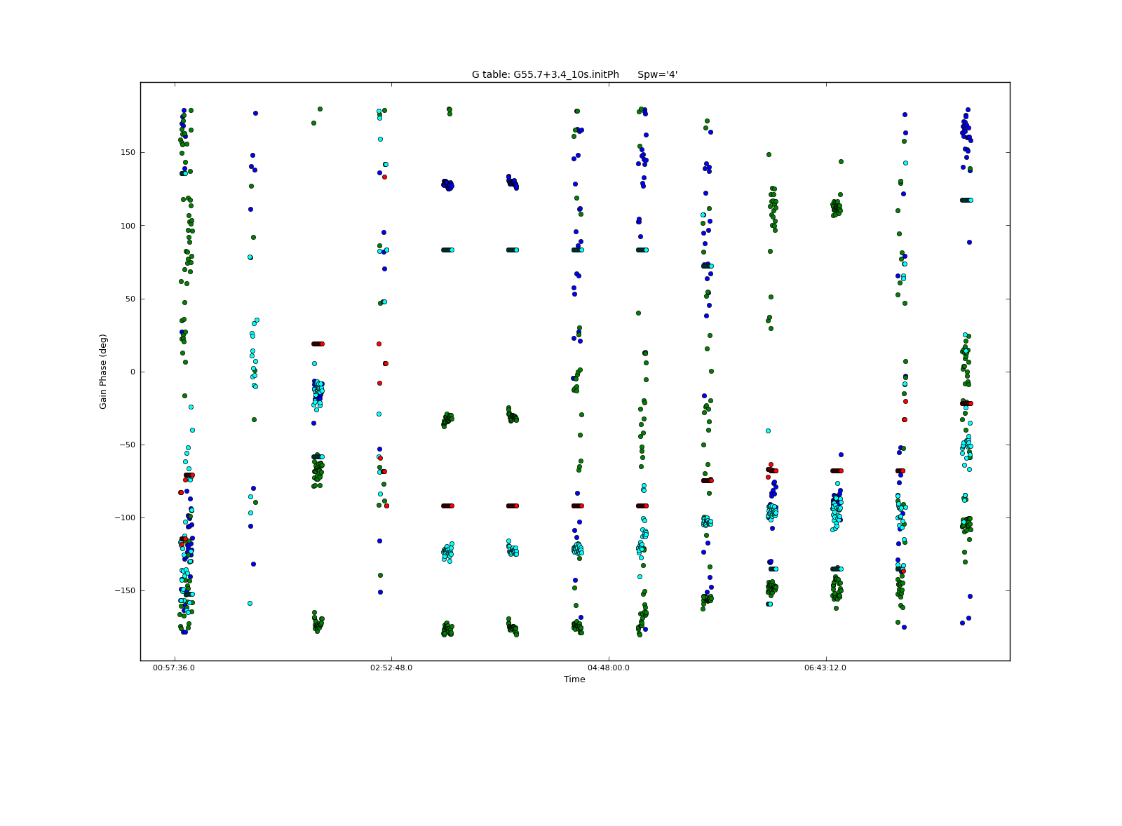
We can inspect the resulting calibration table with plotcal:
# In CASA
plotcal(caltable='G55.7+3.4_10s.initPh', xaxis='time', yaxis='phase',
        iteration='antenna', spw='0', plotrange=[-1,-1,-180,180])
This iterates over antenna for a single spectral window; we can see that the phase does not change much over the course of the observation for SPW 0. We may also iterate over spectral window for a subset of antennas:
# In CASA
plotcal(caltable='G55.7+3.4_10s.initPh', xaxis='time', yaxis='phase',
        iteration='spw', antenna='ea01,ea05,ea24', plotrange=[-1,-1,-180,180])
Clearly, the phases are affected by RFI in some places, especially in SPW 4.
Using this phase information, we create time-averaged bandpass solutions for the phase calibration source:
# In CASA
bandpass(vis='G55.7+3.4_10s.ms', caltable='G55.7+3.4_10s.initBP',
         intent='CALIBRATE_PHASE*', solint='inf',
         combine='scan', refant='ea24', minblperant=3, minsnr=10.0,
         gaintable=['G55.7+3.4_10s.pos', 'G55.7+3.4_10s.initPh'],
         interp=['', 'nearest'], solnorm=False)
- solint='inf', combine='scan': the solution interval of 'inf' will automatically break by scans; this requests that the solution intervals be combined over scans, so that we will get one solution per antenna.
- gaintable=['G55.7+3.4_10s.pos', 'G55.7+3.4_10s.initPh']: we will pre-apply both the corrected antenna position as well as the initial phase solutions.
- interp=['', 'nearest']: by default, gaincal will use linear interpolation for pre-applied calibration. However, we want the nearest phase solution to be used for a given time.
Again, we can see that a number of solutions have been rejected by our choices of minblperant and minsnr.
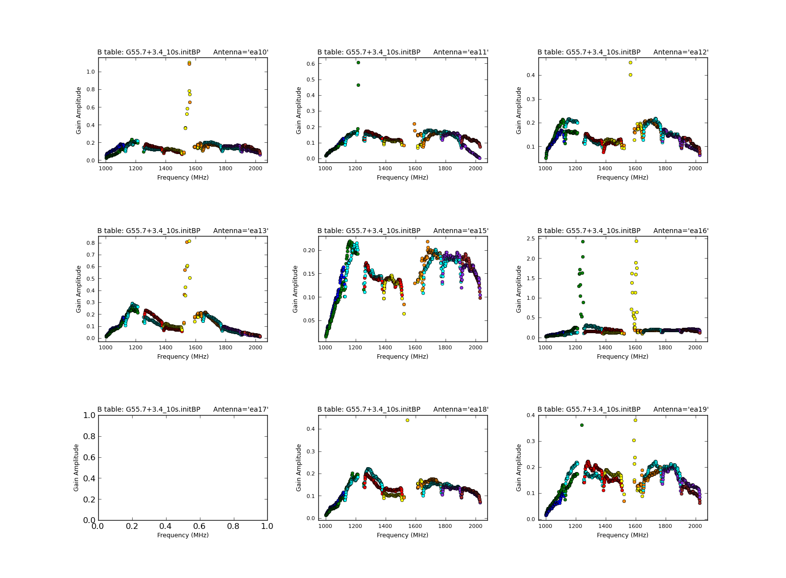
We may plot the bandpasses with plotcal; first looking at the amplitudes:
# In CASA
plotcal(caltable='G55.7+3.4_10s.initBP', xaxis='freq', yaxis='amp',
        iteration='antenna', subplot=331)
- subplot=331: displays 3x3 plots per screen
Also, we can look at the phase solutions:
# In CASA
plotcal(caltable='G55.7+3.4_10s.initBP', xaxis='freq', yaxis='phase',
        iteration='antenna', subplot=331)
We can see that SPW 4 is virtually wiped out by RFI; furthermore, there are channels in SPW 1 that are consistently badly affected. Prior to running any automatic flagging, we will flag these manually. In addition, we will flag the first 9 channels of SPW 0, since this is affected by an issue which causes the noise to be substantially higher:
# In CASA
flagdata(vis='G55.7+3.4_10s.ms', spw='0:0~8,1:41~63,4')
Note that this has created a backup flag file called "flagdata_2". Now we apply the antenna position correction and this bandpass calibration to the data:
# In CASA
applycal(vis='G55.7+3.4_10s.ms',
         gaintable=['G55.7+3.4_10s.pos', 'G55.7+3.4_10s.initBP'],
         calwt=False)
This operation will flag data that correspond to flagged solutions, so applycal makes a backup version of the flags prior to operating on the data -- in this case, it's called "before_applycal_1". Note that running applycal might take a little while, likely around 10 minutes.
To see the corrected data, we can plot the data as we did before, choosing ydatacolumn='corrected' this time:
# In CASA
plotms(vis='G55.7+3.4_10s.ms', scan='30,75,120,165,190,235,303',
       antenna='ea24', xaxis='freq', yaxis='amp', coloraxis='spw',
       iteraxis='scan', ydatacolumn='corrected')
Note that some of the worst RFI is no longer there; also note that the amplitude scale has changed, since the bandpass solutions include amplitude scaling.
Automatic flagging
Now that we have bandpass-corrected data with some of the worst RFI flagged out, we will run flagdata in mode='rflag'. Note that there are many parameters which may be modified:
# In CASA
default flagdata
mode='rflag'
inp
#  flagdata :: All-purpose flagging task based on data-selections and flagging modes/algorithms
vis                 =         ''        #  Name of MS file to flag
mode                =    'rflag'        #  Flagging mode
                                        #   (list/manual/clip/shadow/quack/elevation/tfcrop/rflag/extend/unflag/summary)
     field          =         ''        #  Field names or field index numbers: '' ==> all, field='0~2,3C286'
     spw            =         ''        #  Spectral-window/frequency/channel: '' ==> all, spw='0:17~19'
     antenna        =         ''        #  Antenna/baselines: '' ==> all, antenna ='3,VA04'
     timerange      =         ''        #  Time range: '' ==> all,timerange='09:14:0~09:54:0'
     correlation    =         ''        #  Correlation: '' ==> all, correlation='XX,YY'
     scan           =         ''        #  Scan numbers: '' ==> all
     intent         =         ''        #  Observation intent: '' ==> all, intent='CAL*POINT*'
     array          =         ''        #  (Sub)array numbers: '' ==> all
     uvrange        =         ''        #  UV range: '' ==> all; uvrange ='0~100klambda', default units=meters
     observation    =         ''        #  Observation ID: '' ==> all
     feed           =         ''        #  Multi-feed numbers: Not yet implemented
     ntime          =     'scan'        #  Time-range to use for each chunk (in seconds or minutes)
     combinescans   =      False        #  Accumulate data across scans.
     datacolumn     =     'DATA'        #  Data column on which to operate (data,corrected,model,residual)
     winsize        =          3        #  Number of timesteps in the sliding time window [aips:fparm(1)]
     timedev        =         ''        #  Time-series noise estimate [aips:noise]
     freqdev        =         ''        #  Spectral noise estimate [aips:scutoff]
     timedevscale   =        5.0        #  Threshold scaling for timedev [aips:fparm(9)]
     freqdevscale   =        5.0        #  Threshold scaling for freqdev [aips:fparm(10)]
     spectralmax    =  1000000.0        #  Flag whole spectrum if freqdev is greater than spectralmax [aips:fparm(6)]
     spectralmin    =        0.0        #  Flag whole spectrum if freqdev is less than spectralmin [aips:fparm(5)]

action              =    'apply'        #  Action to perform in MS and/or in inpfile (none/apply/calculate)
     display        =         ''        #  Display data and/or end-of-MS reports at runtime (data/report/both).
     flagbackup     =       True        #  Back up the state of flags before the run

savepars            =      False        #  Save the current parameters to the FLAG_CMD table or to a file
async               =      False        #  If true the taskname must be started using flagdata(...)
Additional information on the algorithm used in RFlag, as well as the other available automatic flagging algorithm in flagdata ("TFCrop"), can be found on this webpage (sections 2.1.6 and 2.1.7).
Following are a set of flagdata commands which have been found to work reasonably well with these data. Please take some time to play with the parameters and the plotting capabilities. Since these runs set display='both' and action='calculate', the flags are displayed but not actually written to the MS. This allows one to try different sets of parameters before actually applying the flags to the data.
Some representative plots are also displayed. Each column displays an individual polarization product; since we're using all four, from left to right are RR, RL, LR, and LL. The first row shows the data with current flags applied, and the second includes the flags generated by flagdata. The x-axis is channel number (the spectral window ID is displayed in the top title) and the y-axis of the first two rows is all integrations included in a time "chunk", set by the ntime parameter. These are the data considered by the RFlag algorithm during its flagging process, and changes in ntime will have some (relatively small) affect on what data are flagged.
Each plot page displays data for a single baseline and time chunk. The buttons at the bottom allow one to step through baseline (backward as well as forward), SPW, scan, and field; "Stop Display" will continue the flagging operation without the GUI, and "Quit" aborts the run.
First, we will run flagdata with mode='rflag', using the default parameter values, for just one source (the supernova remnant) and spectral window (0):
# In CASA
flagdata(vis='G55.7+3.4_10s.ms', mode='rflag', field='2',
         spw='0', datacolumn='corrected',
         action='calculate', display='both',
         flagbackup=False)
While this is clearly picking up some RFI, much is being left untouched (see figure to left, below). After stepping through a few baselines and scans, hit "Quit" to stop the flagger.
Let's try making it more sensitive to deviations from the calculated RMS in frequency, setting both timedevscale and freqdevscale=1.5 (the default is 5.0):
# In CASA
flagdata(vis='G55.7+3.4_10s.ms', mode='rflag', field='2',
         spw='0', datacolumn='corrected',
         freqdevscale=1.5, timedevscale=1.5,
         action='calculate', display='both',
         flagbackup=False)
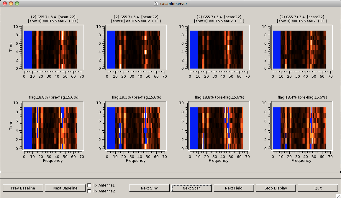
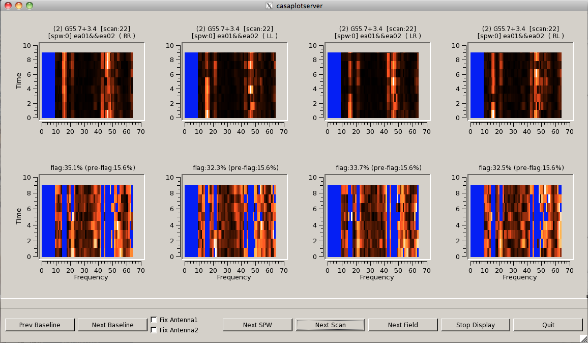
Using a cutoff value of 1.5 sigma may seem a bit extreme, but as you can see from the figure on the right, it does a substantially better job of getting rid of the RFI in the badly affected SPW 0.
We now run flagdata to calculate and apply these flags for all data in SPW 0. Note that this will take a little while, and flags around 20% of the data:
# In CASA
flagdata(vis='G55.7+3.4_10s.ms', mode='rflag',
         spw='0', datacolumn='corrected',
         freqdevscale=1.5, timedevscale=1.5,
         action='apply', display='')
Although RFlag has done a pretty good job of finding the bad data, some still remains. One way to delete it is to use the mode='extend' feature in flagdata, which can extend flags along a chosen axis. First, we will extend the flags across polarization, so if any one polarization is flagged, all data for that time / channel will be flagged:
# In CASA
flagdata(vis='G55.7+3.4_10s.ms', mode='extend',
         spw='0', extendpols=True,
         action='apply', display='')
Now, we will extend the flags in time and frequency, using the "growtime" and "growfreq" parameters. For the data here, the RFlag algorithm seems most likely to miss RFI which should be flagged along more of the time axis, so we will try with growtime=50.0, which will flag all data for a given channel if more than 50% of that channel's time is already flagged, and growfreq=90.0, which will flag the entire spectrum for an integration if more than 90% of the channels in that integration are already flagged.
Again, first just have a look at the flags that will be generated before applying them:
# In CASA
flagdata(vis='G55.7+3.4_10s.ms', mode='extend',
         spw='0', growtime=50.0, growfreq=90.0,
         action='calculate', display='data',
         flagbackup=False)
It still appears to be missing some RFI, but this is also a very badly-affected SPW, so leave it as is for now and run to apply the flags:
# In CASA
flagdata(vis='G55.7+3.4_10s.ms', mode='extend',
         spw='0', growtime=50.0, growfreq=90.0,
         action='apply', display='')
Now, let's work on SPW 1, flipping through time, baseline, and fields to get a sense of how the flagging will go with these parameters:
# In CASA
flagdata(vis='G55.7+3.4_10s.ms', mode='rflag',
         spw='1', datacolumn='corrected',
         freqdevscale=2.0, timedevscale=2.0,
         action='calculate', display='both',
         flagbackup=False)
Unfortunately, this SPW is very badly affected by RFI, and it does not seem possible to flag adequately with the automated task (and probably not by hand, either). In this case, we choose to manually flag the entire SPW:
# In CASA
flagdata(vis='G55.7+3.4_10s.ms', spw='1')
Moving on to SPW 2:
# In CASA
flagdata(vis='G55.7+3.4_10s.ms', mode='rflag',
         spw='2', datacolumn='corrected',
         freqdevscale=5.0, timedevscale=4.0,
         action='calculate', display='both',
         flagbackup=False)
Since the RFI is narrower and more pronounced in this frequency range, we have increased the RMS cutoff for both the time and frequency calculations to avoid over-flagging and deleting good data.
After checking the data and changing the parameters until you're happy, apply these flags:
# In CASA
flagdata(vis='G55.7+3.4_10s.ms', mode='rflag',
         spw='2', datacolumn='corrected',
         freqdevscale=5.0, timedevscale=4.0,
         action='apply')
Again, extend the flags along polarization:
# In CASA
flagdata(vis='G55.7+3.4_10s.ms', mode='extend',
         spw='2', extendpols=True,
         action='apply', display='')
Try extending in frequency and time, as before:
# In CASA
flagdata(vis='G55.7+3.4_10s.ms', mode='extend',
         spw='2', growtime=50.0, growfreq=90.0,
         action='calculate', display='data',
         flagbackup=False)
This looks pretty good, so let's apply it and have a look in plotms:
# In CASA
flagdata(vis='G55.7+3.4_10s.ms', mode='extend',
         spw='2', growtime=50.0, growfreq=90.0,
         action='apply')
plotms(vis='G55.7+3.4_10s.ms', scan='30,75,120,165,190,235,303',
       xaxis='baseline', yaxis='amp', spw='2',
       iteraxis='scan', correlation='rr,ll')
Although we're trying to avoid doing this too much, it appears that there is one baseline which is consistently higher-amplitude than the others, indicating that it's probably contaminated by RFI. Use the plotms tools to identify this baseline, which turns out to be ea04 and ea16, and flag it:
# In CASA
flagdata(vis='G55.7+3.4_10s.ms', antenna='ea04&ea16',
         spw='2')
We could have narrowed this further by channel and perhaps time, but remember: this tutorial is about the quick-and-dirty way of flagging data! With this in mind, we move on to SPW 3. Note that this time, we only look at data from the supernova remnant (target) field.
# In CASA
flagdata(vis='G55.7+3.4_10s.ms', mode='rflag',
         spw='3', datacolumn='corrected', field='2',
         freqdevscale=5.0, timedevscale=4.0,
         action='calculate', display='data',
         flagbackup=False)
The parameters we used for SPW 2 seem to work well for SPW 3 also. Go ahead and flag, then extend as before:
# In CASA
flagdata(vis='G55.7+3.4_10s.ms', mode='rflag',
         spw='3', datacolumn='corrected',
         freqdevscale=5.0, timedevscale=4.0,
         action='apply')
flagdata(vis='G55.7+3.4_10s.ms', mode='extend',
         spw='3', extendpols=True,
         action='apply')
flagdata(vis='G55.7+3.4_10s.ms', mode='extend',
         spw='3', growtime=50.0, growfreq=90.0,
         action='apply')
Recall that we already deleted SPW 4 due to bad RFI, so we only have 5-7 remaining. SPWs 5 and 6 have similar RFI properties to 2 and 3, so let's use the same RFlag parameters for these (feel free to play with this a bit yourself, if you like, to try to optimize):
# In CASA
flagdata(vis='G55.7+3.4_10s.ms', mode='rflag',
         spw='5~6', datacolumn='corrected',
         freqdevscale=5.0, timedevscale=4.0,
         action='apply')
flagdata(vis='G55.7+3.4_10s.ms', mode='extend',
         spw='5~6', extendpols=True,
         action='apply')
flagdata(vis='G55.7+3.4_10s.ms', mode='extend',
         spw='5~6', growtime=50.0, growfreq=90.0,
         action='apply')
However, SPW 7 is a bit more affected, and we may wish to use a somewhat lower threshold to catch all the RFI. First, try with the same parameters:
# In CASA
flagdata(vis='G55.7+3.4_10s.ms', mode='rflag',
         spw='7', datacolumn='corrected', field='2',
         freqdevscale=5.0, timedevscale=4.0,
         action='calculate', display='data',
         flagbackup=False)
Indeed, this seems to be missing a lot of the RFI. Try less stringent limits:
# In CASA
flagdata(vis='G55.7+3.4_10s.ms', mode='rflag',
         spw='7', datacolumn='corrected', field='2',
         freqdevscale=1.0, timedevscale=1.0,
         action='calculate', display='data',
         flagbackup=False)
This looks pretty good. Check the calibrator sources to be sure it works for them as well:
# In CASA
flagdata(vis='G55.7+3.4_10s.ms', mode='rflag',
         spw='7', datacolumn='corrected', field='1',
         freqdevscale=1.0, timedevscale=1.0,
         action='calculate', display='data',
         flagbackup=False)
flagdata(vis='G55.7+3.4_10s.ms', mode='rflag',
         spw='7', datacolumn='corrected', field='3',
         freqdevscale=1.0, timedevscale=1.0,
         action='calculate', display='data',
         flagbackup=False)
These seem reasonable as well, though it's apparent that 3C147 was very affected, possibly because of its low elevation at the time of the observation. Apply and extend the flags:
# In CASA
flagdata(vis='G55.7+3.4_10s.ms', mode='rflag',
         spw='7', datacolumn='corrected',
         freqdevscale=1.0, timedevscale=1.0,
         action='apply')
flagdata(vis='G55.7+3.4_10s.ms', mode='extend',
         spw='7', extendpols=True,
         action='apply')
flagdata(vis='G55.7+3.4_10s.ms', mode='extend',
         spw='7', growtime=50.0, growfreq=90.0,
         action='apply')
Evaluating results & further manual flagging
Now, we will use flagdata to see a summary of how much data we have flagged:
# In CASA
flagInfo = flagdata(vis='G55.7+3.4_10s.ms', mode='summary')
Using the information stored in the flagInfo Python dictionary, we can calculate and print out some interesting statistics:
# In CASA
print("\n %2.1f%% of G55.7+3.4, %2.1f%% of 3C147, and %2.1f%% of J1925+2106 are flagged. \n" % (100.0 * flagInfo['field']['G55.7+3.4']['flagged'] / flagInfo['field']['G55.7+3.4']['total'], 100.0 * flagInfo['field']['0542+498=3C147']['flagged'] / flagInfo['field']['0542+498=3C147']['total'], 100.0 * flagInfo['field']['J1925+2106']['flagged'] / flagInfo['field']['J1925+2106']['total']))
print("Spectral windows are flagged as follows:")
for spw in range(0,8):
     print("SPW %s: %2.1f%%" % (spw, 100.0 * flagInfo['spw'][str(spw)]['flagged'] / flagInfo['spw'][str(spw)]['total']))
So, as a result of the flagging thus far, we have sacrificed a bit over half of all the data. Let's see how well it has been cleaned up, using plotms:
# In CASA
plotms(vis='G55.7+3.4_10s.ms', scan='165', spw='0,2~3,5~7',
       antenna='ea24', xaxis='freq', yaxis='amp',
       correlation='rr,ll', coloraxis='spw')
Unfortunately, despite our best autoflagging efforts, SPW 0 still looks pretty bad. (Take heart -- even the by-hand flagging did not work out well for this one.) So, we will flag the rest of SPW 0:
# In CASA
flagdata(vis='G55.7+3.4_10s.ms', spw='0')

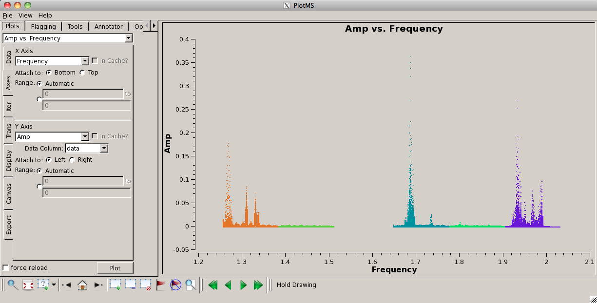
After this is complete, refresh the plotms window using Shift + Plot. This generates the plot to the left. Just to compare with the unflagged data, we will restore the original flags, and have a look at the same slice. Be sure to save the current flags first!
# In CASA
flagmanager(vis='G55.7+3.4_10s.ms', mode='save',
            versionname='after_autoflagging_1')
flagmanager(vis='G55.7+3.4_10s.ms', mode='restore',
            versionname='flagdata_1')
plotms(vis='G55.7+3.4_10s.ms', scan='165', spw='2~3,5~7',
       antenna='ea24', xaxis='freq', yaxis='amp',
       correlation='rr,ll', coloraxis='spw')
The pre-flagging plot is shown on the right. Clearly, a lot of the RFI has been excised. Restore the flags:
# In CASA
flagmanager(vis='G55.7+3.4_10s.ms', mode='restore',
            versionname='after_autoflagging_1')
Other instructive ways to view the data are by baseline and uv-distance. Note that we're plotting all baselines in these plots, rather than just baselines to ea24 as before.
# In CASA
plotms(vis='G55.7+3.4_10s.ms', scan='30,75,120,165,190,235,303',
       xaxis='baseline', yaxis='amp', spw='2~3,5~7', iteraxis='spw',
       correlation='rr,ll', coloraxis='antenna1')
No particular baselines look bad enough to flag outright, so we will leave this as is. Feel free to do some more flagging if you like. Now, let's plot as a function of uv-distance:
# In CASA
plotms(vis='G55.7+3.4_10s.ms', scan='30,75,120,165,190,235,303',
       xaxis='uvdist', yaxis='amp', spw='2~3,5~7', iteraxis='spw',
       correlation='rr,ll', coloraxis='antenna1')
Again, nothing really sticks out as obviously in need of flagging. Clearly, there is still some residual RFI left here and there -- however, for the purposes of this tutorial, we will accept the current state of the flags and move on. Feel free to hunt and excise some more, if desired.
Calibrating data
Now that we are satisfied with the RFI excision, we will move on to the calibration stage.
Setting the flux density scale
Since we will be using 3C147 as the source of the absolute flux scale for this observation, we must first run setjy to set the appropriate model amplitudes for this source.
If the flux calibrator is spatially resolved, it is necessary to include a model image as well. Although 3C147 is not resolved at L-band in D configuration, we include the model image here for completeness.
First, we use the listmodimages parameter to find the model image path:
# In CASA
setjy(vis='G55.7+3.4_10s.ms', listmodels=True)
This lists any images in the current working directory as well as images in CASA's repository. In this second list, we see that there is "3C147_L.im", which is appropriate for our flux calibrator and band, and that it is in the directory "/usr/lib64/casapy/release/nrao/VLA/CalModels". We can optionally give the full path of the model image, but setjy should now be able to locate it by name alone:
# In CASA
setjy(vis='G55.7+3.4_10s.ms', field='0542*', scalebychan=True,
      spw='2~3,5~7', modimage='3C147_L.im')
- scalebychan=True: scales the model flux density value for each channel. By default, only one value per spectral window is calculated.
Bandpass calibration
We will follow the same procedure outlined above for calculating the antenna bandpasses, except that this time, we will use the actual designated bandpass calibration source, 3C147. Although the phase calibration source has the advantage of having been observed throughout the run, it has an unknown spectrum which could introduce amplitude slopes to each spectral window.
# In CASA
gaincal(vis='G55.7+3.4_10s.ms', intent='*BANDPASS*',
        caltable='G55.7+3.4_10s.initPh.2',
        spw='3;5~6:30~33,2:32~35,7:50~53',
        solint='int', refant='ea24',
        minblperant=3, minsnr=3.0, calmode='p',
        gaintable='G55.7+3.4_10s.pos')
Unfortunately, you will notice a lot of message that read "Insufficient unflagged antennas to proceed with this solve" for SPW 7. This indicates that too much data have been flagged to perform the gaincal operation. This also suggests that the spectral window is too badly affected by RFI to be useful for imaging -- so, we will flag the rest of the SPW before continuing with further analysis:
# In CASA
flagdata(vis='G55.7+3.4_10s.ms', spw='7')
Now, on to creating the bandpass calibration for the remaining spectral windows:
# In CASA
bandpass(vis='G55.7+3.4_10s.ms', caltable='G55.7+3.4_10s.bPass',
         intent='*BANDPASS*', solint='inf', spw='2~3,5~6',
         combine='scan', refant='ea24', minblperant=3, minsnr=10.0,
         gaintable=['G55.7+3.4_10s.pos','G55.7+3.4_10s.initPh.2'],
         interp=['', 'nearest'], solnorm=False)
- solint='inf', combine='scan': again, the solution interval of 'inf' will automatically break by scans; this requests that the solution intervals be combined over scans, so that we will get one solution per antenna.
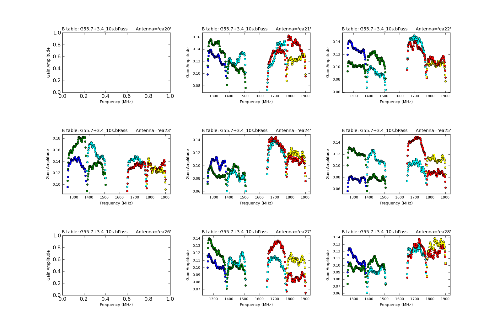
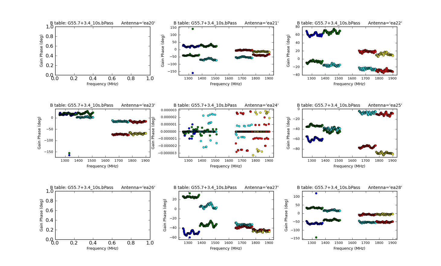
Note that since we have flagged out the vast majority of the RFI-affected data, there are many fewer failed solutions. Again, we can plot the calculated bandpasses to check that they look reasonable:
# In CASA
plotcal(caltable='G55.7+3.4_10s.bPass', xaxis='freq', yaxis='amp',
        iteration='antenna', subplot=331)
#
plotcal(caltable='G55.7+3.4_10s.bPass', xaxis='freq', yaxis='phase',
        iteration='antenna', subplot=331)
Don't let the apparently odd-looking phases for ea24 fool you -- check the scale! Remember, this is our reference antenna.
Gain calibration
Next, we will calculate the per-antenna gain solutions. Since this is low-frequency data, we do not expect substantial variations over short timescales, so we calculate one solution per scan (using "solint='inf'"):
# In CASA
gaincal(vis='G55.7+3.4_10s.ms', caltable='G55.7+3.4_10s.phaseAmp',
        intent='*PHASE*,*AMPLI*',
        spw='2~3,5~6', solint='inf', refant='ea24', minblperant=3,
        minsnr=10.0, gaintable=['G55.7+3.4_10s.pos','G55.7+3.4_10s.bPass'])
- solint='inf': we request one solution per scan.
Plot these solutions as a function of time, iterating over antenna:
# In CASA
plotcal(caltable='G55.7+3.4_10s.phaseAmp', xaxis='time', yaxis='amp',
        iteration='antenna')

plotcal(caltable='G55.7+3.4_10s.phaseAmp', xaxis='time', yaxis='phase',
        iteration='antenna')
Flux scaling the gain solutions
Now that we have a complete set of gain solutions, we must scale the phase calibrator's absolute flux correctly, using 3C147 as our reference source. To do this, we run fluxscale on the gain table we just created, which will write a new, flux-corrected gain table:
# In CASA
myFlux = fluxscale(vis='G55.7+3.4_10s.ms', caltable='G55.7+3.4_10s.phaseAmp',
                   fluxtable='G55.7+3.4_10s.phaseAmp.fScale', reference='3')
Note that the myFlux Python dictionary will contain information about the scaled fluxes and fitted spectrum. The logger will display information about the flux density it has deduced for J1925+2106:
Found reference field(s): 0542+498=3C147
Found transfer field(s):  J1925+2106
Flux density for J1925+2106 in SpW=0 is:  INSUFFICIENT DATA
Flux density for J1925+2106 in SpW=1 is:  INSUFFICIENT DATA
Flux density for J1925+2106 in SpW=2 is: 1.46169 +/- 0.0285038 (SNR = 51.2806, N = 40)
Flux density for J1925+2106 in SpW=3 is: 1.53198 +/- 0.0250909 (SNR = 61.057, N = 40)
Flux density for J1925+2106 in SpW=4 is:  INSUFFICIENT DATA
Flux density for J1925+2106 in SpW=5 is: 1.69898 +/- 0.024897 (SNR = 68.2404, N = 40)
Flux density for J1925+2106 in SpW=6 is: 1.75286 +/- 0.0265399 (SNR = 66.0463, N = 40)
Flux density for J1925+2106 in SpW=7 is:  INSUFFICIENT DATA
Fitted spectrum for J1925+2106 with fitorder=1: Flux density = 1.60707 +/- 0.00474563 (freq=1.50187 GHz) spidx=0.539949 +/- 0.0222143
The flux density listed in the VLA Calibrator Manual for this source is around the same magnitude:
1925+211   J2000  A 19h25m59.605370s  21d06'26.162180"  Aug01
1923+210   B1950  A 19h23m49.792400s  21d00'23.305000"
-----------------------------------------------------
BAND        A B C D    FLUX(Jy)    UVMIN(kL)  UVMAX(kL)
=====================================================
 20cm    L  P S S S       1.30                       visplot
So we should be satisfied that our calibration up to this point is reasonable.
Applying calibration
Finally, we must apply the calibration to our data. To do this, we run applycal in two stages: the first is to self-calibrate our calibration sources; the second, to apply calibration to the supernova remnant. These must be done separately, since we want to use "nearest" interpolation for the self-calibration and "linear" for the application to the science target:
# In CASA
applycal(vis='G55.7+3.4_10s.ms', spw='2~3,5~6', intent='*TARGET*',
         gaintable=['G55.7+3.4_10s.pos','G55.7+3.4_10s.bPass', \
                    'G55.7+3.4_10s.phaseAmp.fScale'], calwt=False)
#
applycal(vis='G55.7+3.4_10s.ms', spw='2~3,5~6', intent='*PHASE*,*AMPLI*',
         gaintable=['G55.7+3.4_10s.pos','G55.7+3.4_10s.bPass', \
                    'G55.7+3.4_10s.phaseAmp.fScale'], \
         calwt=False, interp=['','nearest','nearest'])
Plotting calibrated data
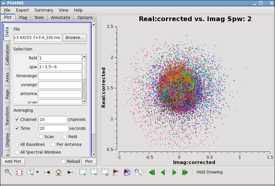
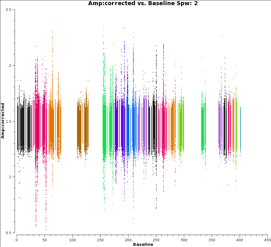
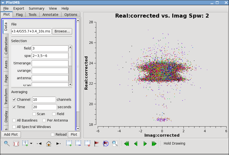
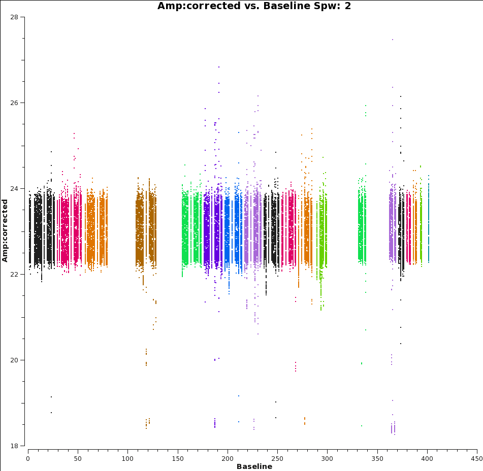
To check that everything has truly proceeded as well as we would like, this is a good time to look at the calibrated data in plotms. A very useful way to check the goodness of calibration is to plot the corrected amplitude vs. corrected phase (which should look like a tight ball for a point source, and will have organized structure if the source is resolved), and corrected amplitude vs. baseline, which should be a flat line of points for a point source, and will reveal any lingering antenna-based problems. For a resolved source, it may be more instructive to plot corrected amplitude vs. uv-distance.
# In CASA
plotms(vis='G55.7+3.4_10s.ms', field='1', xaxis='phase', yaxis='amp',
       xdatacolumn='corrected', ydatacolumn='corrected', coloraxis='antenna1',
       avgchannel='10', avgtime='20', correlation='rr,ll', iteraxis='spw',
       spw='2~3,5~6')
#
plotms(vis='G55.7+3.4_10s.ms', field='1', xaxis='baseline', yaxis='amp',
       xdatacolumn='corrected', ydatacolumn='corrected', coloraxis='antenna1',
       avgchannel='10', avgtime='20', correlation='rr,ll', iteraxis='spw',
       spw='2~3,5~6')
#
plotms(vis='G55.7+3.4_10s.ms', field='3', xaxis='phase', yaxis='amp',
       xdatacolumn='corrected', ydatacolumn='corrected', coloraxis='antenna1',
       avgchannel='10', avgtime='20', correlation='rr,ll', iteraxis='spw',
       spw='2~3,5~6')
#
plotms(vis='G55.7+3.4_10s.ms', field='3', xaxis='baseline', yaxis='amp',
       xdatacolumn='corrected', ydatacolumn='corrected', coloraxis='antenna1',
       avgchannel='10', avgtime='20', correlation='rr,ll', iteraxis='spw',
       spw='2~3,5~6')
Splitting out data for G55.7+3.4
Now that we are satisfied with the calibration, we will create a new MS which contains only the corrected data for G55.7+3.4 using the task split. This will substantially reduce the size of the MS, and will speed up the imaging process. We can also drop the polarization products since they have not been calibrated and will not be used for imaging.
# In CASA
split(vis='G55.7+3.4_10s.ms', field='2', keepflags=False,
      outputvis='G55.7+3.4.calib.ms', datacolumn='corrected',
      spw='2~3,5~6', correlation = 'rr,ll')
Imaging
The size of the primary beam is 45 arcmin divided by the observed frequency in GHz, or around 30 arcmin. Since the observation was taken in D-configuration, we can check the Observational Status Summary's section on VLA resolution to find that the synthesized beam will be around 44 arcsec. We want to oversample the synthesized beam by a factor of around five, so we will use a cell size of 8 arcsec.
Since this field contains bright point sources significantly outside the primary beam, we will create images that are 170 arcminutes on a side, or almost 6 x the size of the primary beam. This is ideal for showcasing both the problems inherent in such wide-band, wide-field imaging, as well as some of the solutions currently available in CASA to deal with these issues.
First, it's worth considering why we are even interested in sources which are far outside the primary beam. This is mainly due to the fact that the EVLA, with its wide bandwidth capabilities, is quite sensitive even far from phase center -- for example, at our observing frequencies in L-band, the primary beam gain is as much as 10% around 1 degree away. That means that any imaging errors for these far-away sources will have a significant impact on the image rms at phase center. The error due to a source at distance R can be parametrized as:
[math]\displaystyle{ \Delta(S) = S(R) \times PB(R) \times PSF(R) }[/math]
So, for R = 1 degree, source flux S(R) = 1 Jy, [math]\displaystyle{ \Delta(S) }[/math] = 1 mJy − 100 [math]\displaystyle{ {\mu} }[/math]Jy. Clearly, this will be a source of significant error.
Multi-scale clean
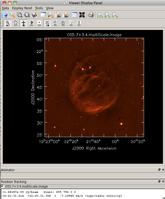
Since G55.7+3.4 is an extended source with many spatial scales, the most basic (yet still reasonable) imaging procedure is to use clean with multiple scales. As is suggested, we will use a set of scales (which are expressed in units of the requested pixel, or cell, size) which are representative of the scales that are present in the data, including a zero-scale for point sources.
Note that interrupting clean by Ctrl+C may corrupt your visibilities -- you may be better off choosing to let clean finish. We are currently implementing a command that will nicely exit to prevent this from happening, but for the moment try to avoid Ctrl+C.
# In CASA
clean(vis='G55.7+3.4.calib.ms', imagename='G55.7+3.4.multiScale',
      imsize=1280, cell='8arcsec', multiscale=[0,6,10,30,60],
      interactive=False, niter=1000,  weighting='briggs',
      stokes='I', threshold='0.1mJy', usescratch=F, imagermode='csclean')
viewer('G55.7+3.4.multiScale.image')
- imagename='G55.7+3.4.multiScale': the root filename used for the various clean outputs. These include the final image (<imagename>.image), the relative sky sensitivity over the field (<imagename>.flux), the point-spread function (also known as the dirty beam; <imagename>.psf), the clean components (<imagename>.model), and the residual image (<imagename>.residual).
- imsize=1280: the image size in number of pixels. Note that entering a single value results in a square image with sides of this value.
- cell='8arcsec': the size of one pixel; again, entering a single value will result in a square pixel size.
- multiscale=[0,6,10,30,60]: a set of scales on which to clean. Since these are in units of the pixel size, we are requesting scales of 0 (a point source), 48, 80, 240, and 480 arcseconds. Note that 16 arcminutes (960 arcseconds) roughly corresponds to the size of G55.7+3.4.
- interactive=False: we will let clean use the entire field for placing model components. Alternatively, you could try using interactive=True, and create regions to constrain where components will be placed. However, this is a very complex field, and creating a region for every bit of diffuse emission as well as each point source can quickly become tedious.
- niter=1000: this controls the number of iterations clean will do in the minor cycle.
- weighting='briggs': use Briggs weighting with a robustness parameter of 0 (halfway between uniform and natural weighting).
- calready=F: do not write the model visibilities to the model data column (only needed for self-calibration)
- imagermode='csclean': use the Cotton-Schwab clean algorithm
- stokes='I': since we have not done any polarization calibration, we only create a total-intensity image.
- threshold='0.1mJy': threshold at which the cleaning process will halt; i.e. no clean components with a flux less than this value will be created. This is meant to avoid cleaning what is actually noise (and creating an image with an artificially low rms). It is advisable to set this equal to the expected rms, which can be estimated using the EVLA exposure calculator. However, in our case, this is a bit difficult to do, since we have lost a hard-to-estimate amount of bandwidth due to flagging, and there is also some residual RFI present. Therefore, we choose 0.1 mJy as a relatively conservative limit.
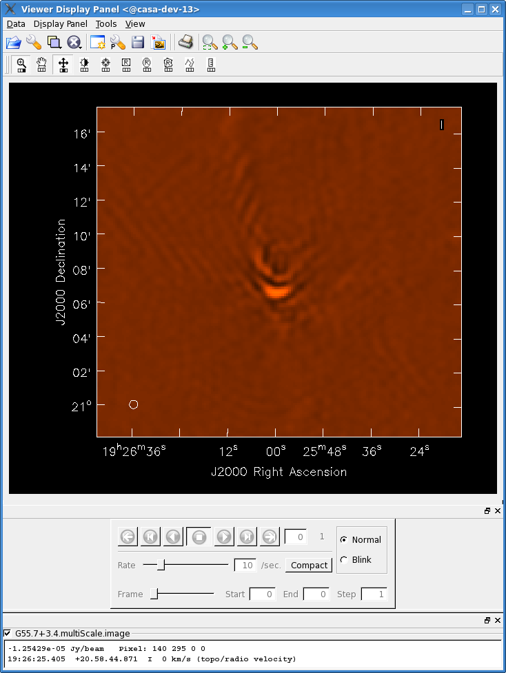
This is the fastest of the imaging techniques described here (it will probably take less than ten minutes to complete), but it's easy to see that there are artifacts in the resulting image. For example, use the viewer to explore the point sources near the edge of the field. Some have prominent arcs, as well as spots in a six-pointed pattern surrounding them. Next we will explore some more advanced imaging techniques to mitigate these artifacts.
Multi-scale, wide-field clean
The next clean algorithm we will employ is W-projection, which is a wide-field imaging technique that takes into account the non-coplanarity of the baselines as a function of distance from the phase center. For more details on the motivation for this correction, as well as the algorithm itself, see "The Noncoplanar Baselines Effect in Radio Interferometry: The W-Projection Algorithm".
# In CASA
clean(vis='G55.7+3.4.calib.ms', imagename='G55.7+3.4.MS.wProj',
      gridmode='widefield', imsize=1280, cell='8arcsec',
      wprojplanes=128, multiscale=[0,6,10,30,60],
      interactive=False, niter=1000,  weighting='briggs',
      stokes='I', threshold='0.1mJy', usescratch=F, imagermode='csclean')
viewer('G55.7+3.4.MS.wProj.image')
- gridmode='widefield': use the W-projection algorithm.
- wprojplanes=128: the number of W-projection planes to use for deconvolution; 128 is the minimum recommended number.
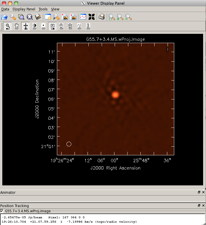
This will take longer than the previous imaging round (likely around 15 minutes); however, the resulting image has noticeably fewer artifacts. In particular, compare the same outlier source in the W-projected image with the multi-scale-only image: note that the swept-back arcs have disappeared. There are still some obvious imaging artifacts remaining, though.
Multi-scale, multi-frequency synthesis
Another consequence of simultaneously imaging the wide fractional bandwidths available with the EVLA is that the primary beam has substantial frequency-dependent variation over the observing band. If this is not accounted for, it will lead to imaging artifacts and compromise the achievable image rms.
If sources which are being imaged have intrinsically flat spectra, this will not be a problem. However, most astronomical objects are not flat-spectrum sources, and without any estimation of the intrinsic spectral properties, the fact that the primary beam is twice as large at 2 than at 1 GHz will have substantial consequences.
The Multi-Scale Multi-Frequency-Synthesis (MS-MFS) algorithm provides the ability to simultaneously image and fit for the intrinsic source spectrum. The spectrum is approximated using a polynomial in frequency, with the degree of the polynomial as a user-controlled parameter.
# In CASA
clean(vis='G55.7+3.4.calib.ms', imagename='G55.7+3.4.MS.MFS',
      imsize=1280, cell='8arcsec', mode='mfs', nterms=2,
      multiscale=[0,6,10,30,60],
      interactive=False, niter=1000,  weighting='briggs',
      stokes='I', threshold='0.1mJy', usescratch=F, imagermode='csclean')
viewer('G55.7+3.4.MS.MFS.image.tt0')
viewer('G55.7+3.4.MS.MFS.image.alpha')
- nterms=2:the number of Taylor terms to be used to model the frequency dependence of the sky emission. Note that the speed of the algorithm will depend on the value used here (more terms will be slower); of course, the image fidelity will improve with a larger number of terms (assuming the sources are sufficiently bright to be modeled more completely).
This will take a little while (likely around 30 minutes), so it would probably be a good time to have coffee or chat about EVLA data reduction with your neighbor at this point.
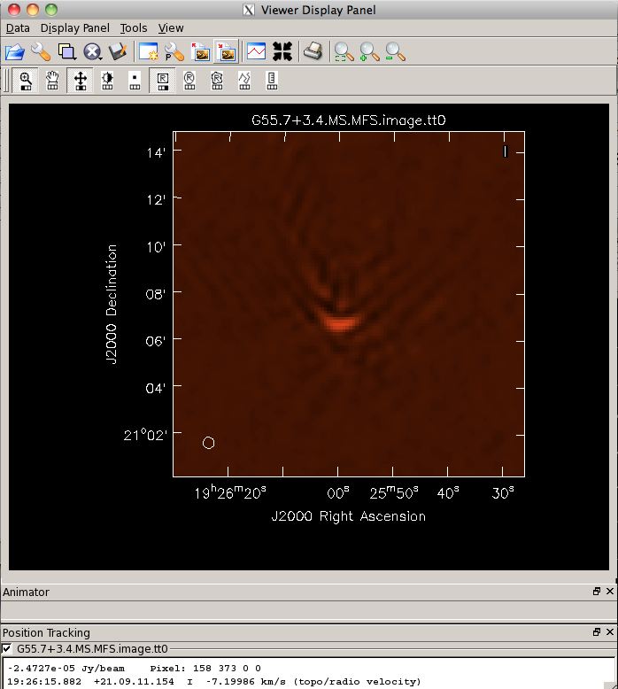
When clean is done <imagename>.image.tt0 will contain a total intensity image; <imagename>.image.alpha will contain an image of the spectral index in regions where there is sufficient signal-to-noise. For more information on the multi-frequency synthesis mode and its outputs, see the CASA cookbook. Inspect the brighter point sources in the field. You will notice that some of the artifacts which had been symmetric around the sources themselves are now gone; however, since we did not use W-projection this time, there are still strong features related to the non-coplanar baseline effects still apparent.
Multi-scale, multi-frequency, wide-field clean
Finally, we will combine the W-projection and MS-MFS algorithms to simultaneously account for both of the effects. Be forewarned -- these imaging runs will take a while, and it's best to start them running and then move on to other things. In testing, both of these runs (on the auto- and by-hand-flagged data) took around an hour.
First, we will image the autoflagged data. Using the same parameters for the individual-algorithm images above, but combined into a single clean run, we have:
# In CASA
clean(vis='G55.7+3.4.calib.ms', imagename='G55.7+3.4.MS.MFS.wProj',
      gridmode='widefield', imsize=1280, cell='8arcsec', mode='mfs',
      nterms=2, wprojplanes=128, multiscale=[0,6,10,30,60],
      interactive=False, niter=1000,  weighting='briggs',
      stokes='I', threshold='0.1mJy', usescratch=F, imagermode='csclean')
viewer('G55.7+3.4.MS.MFS.wProj.image.tt0')
viewer('G55.7+3.4.MS.MFS.wProj.image.alpha')
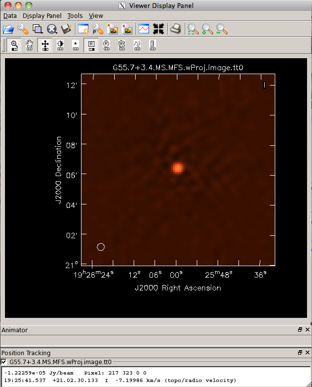
Again, looking at the same outlier source, we can see that the major sources of error have been removed, although there are still some residual artifacts. One possible source of error is the time-dependent variation of the primary beam; another is the fact that we have only used nterms=2, which may not be sufficient to model the spectra of some of the point sources.
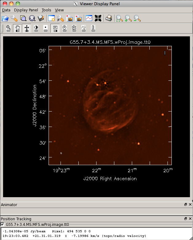
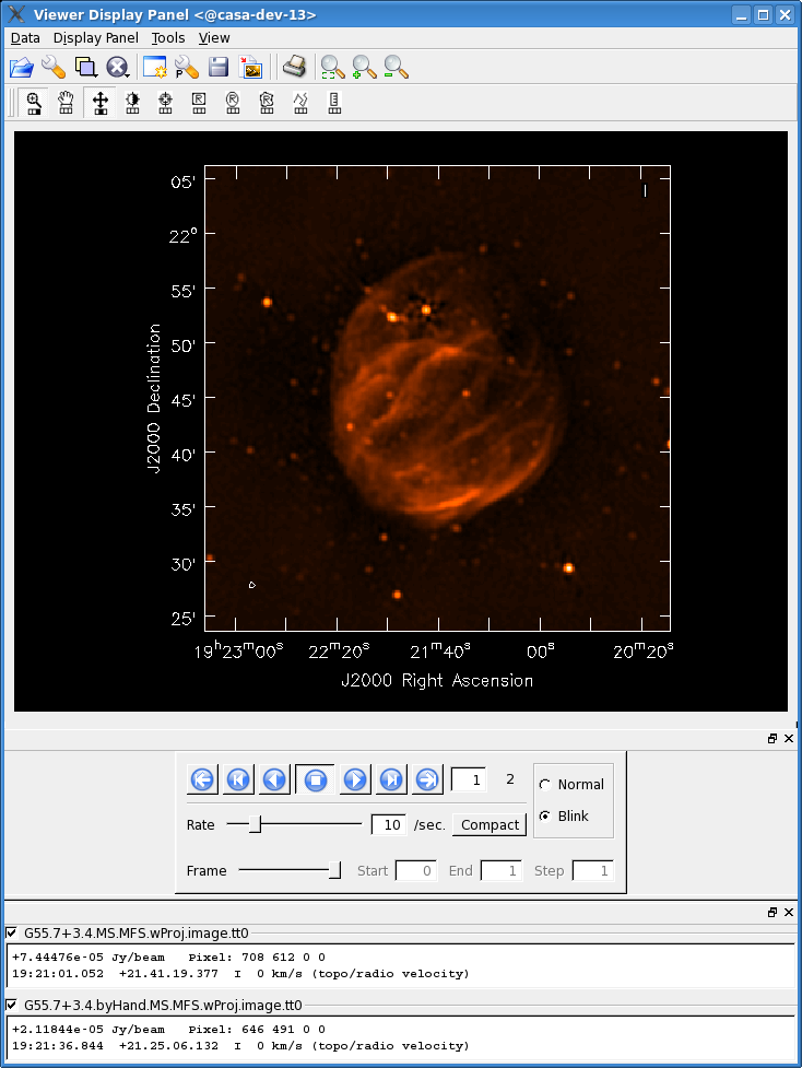
We can compare the resulting image with one that was created from an MS that was flagged by hand, rather than with the automatic flagging routines. While it's clear that this is a superior image, the one that we have created with autoflagging is impressive, considering that the by-hand flagging took a number of weeks, and the autoflagging can be done in a matter of days (or hours, if one knows exactly what parameters to use).
Ultimately, it isn't too surprising that there was still some RFI present in our auto-flagged data, since we were able to see this with plotms. It's also possible that the auto-flagging overflagged some portions of the data, also leading to a reduction in the achievable image rms.
Last checked on CASA Version 4.1.0.