Baseband Stitching

Overview

In order to maintain constant rms noise across an observed frequency range, one may "overlap" EVLA basebands, offsetting one by 0.5 times the subband width. This way, the decreased sensitivity at subband edges can be edited out, and these frequency ranges replaced with data from the other baseband.

The contributed task stitch can be used to make this process simpler. Given a basic set of inputs, it will select channel ranges for each spectral window, which can then be used to run split to create a new measurement set (MS) (stitch can also run split, further simplifying things).

Here, we demonstrate the use of the stitch task. For information on reducing the data after running stitch, see the other CASA Guides EVLA tutorials — the data can be treated in the standard way.

Obtaining and installing stitch

First, you will need to download two files that are needed to build the task:

File:Task stitch.py

File:Stitch.xml

Because of a quirk in the way Wiki stores files, you need to rename these to no longer have capitalized first letters, task_stitch.py and stitch.xml. Next, run buildmytasks to build the needed files for the task. This can either be done in CASA, or in a UNIX shell. You must be inside the directory where you have saved the files.

# In CASA
!buildmytasks

or:

# In the shell
buildmytasks

Once this completes, import the task into CASA:

# In CASA
execfile('mytasks.py')

You should now be able to look at the help and parameter listings of stitch:

# In CASA
inp stitch

#  stitch :: Stitches together desired pieces of overlapping basebands.
vis                 =         ''        #  Name of input measurement set
baseband1           =         []        #  List of first and last spectral windows in lower-frequency baseband (e.g.,
                                        #   [2,9])
baseband2           =         []        #  List of first and last spectral windows in higher-frequency baseband (e.g.,
                                        #   [10,17])
startchan           =         10        #  Starting channel number for lower baseband spectral windows
numchan             =         40        #  Number of channels to use in lower baseband spectral windows
dosplit             =       True        #  Split out selected data to a new MS?
     outputvis      =         ''        #  Name of output measurement set
     datacolumn     = 'corrected'       #  Which data column(s) to split out
     field          =         ''        #  Select field using ID(s) or name(s)
     correlation    =         ''        #  Select correlations
     keepflags      =      False        #  If practical, keep *completely flagged rows* instead of dropping them.

async               =      False        #  If true the taskname must be started using stitch(...)

and

# In CASA
help stitch

Inspecting data and choosing channel range

For the purposes of this guide, we are using EVLA test data that was taken in the overlapping subband mode. This dataset may be found in the EVLA Data Archive; the archive file id is TVER0002_sb2557689_1.55517.018916574074. Here, we have imported it to an MS called overlapSubband.ms.

To start with, we have a look at the data with listobs:

# In CASA:
listobs('overlapSubband.ms')

The most important part of the output is the spectral window information:

Spectral Windows: (18 unique spectral windows and 1 unique polarization setups)

 SpwID  #Chans Frame Ch1(MHz)    ChanWid(kHz)  TotBW(kHz)  Corrs          
 0          64 TOPO  4736        2000          128000      RR  RL  LR  LL  
 1          64 TOPO  7836        2000          128000      RR  RL  LR  LL  
 2          64 TOPO  4488        2000          128000      RR  RL  LR  LL  
 3          64 TOPO  4616        2000          128000      RR  RL  LR  LL  
 4          64 TOPO  4744        2000          128000      RR  RL  LR  LL  
 5          64 TOPO  4872        2000          128000      RR  RL  LR  LL  
 6          64 TOPO  5000        2000          128000      RR  RL  LR  LL  
 7          64 TOPO  5128        2000          128000      RR  RL  LR  LL  
 8          64 TOPO  5256        2000          128000      RR  RL  LR  LL  
 9          64 TOPO  5384        2000          128000      RR  RL  LR  LL  
 10         64 TOPO  4552        2000          128000      RR  RL  LR  LL  
 11         64 TOPO  4680        2000          128000      RR  RL  LR  LL  
 12         64 TOPO  4808        2000          128000      RR  RL  LR  LL  
 13         64 TOPO  4936        2000          128000      RR  RL  LR  LL  
 14         64 TOPO  5064        2000          128000      RR  RL  LR  LL  
 15         64 TOPO  5192        2000          128000      RR  RL  LR  LL  
 16         64 TOPO  5320        2000          128000      RR  RL  LR  LL  
 17         64 TOPO  5448        2000          128000      RR  RL  LR  LL  

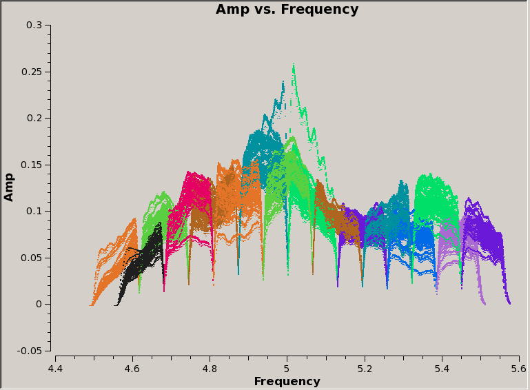
For this observation, we can see that spectral windows 0 and 1 are used for the "dummy" scans, then science data were taken in SPW 2-17. Furthermore, SPW 2-9 are contiguous and in the first baseband, then the frequency jumps back down again, and SPW 10-17 (second baseband) are shifted by half a SPW up in frequency relative to the first baseband. We can also see this by plotting the data:

# In CASA:
plotms(vis='overlapSubband.ms', field='1', antenna='ea21', xaxis='freq',
       yaxis='amp', coloraxis='spw', correlation='rr', avgtime='30s')

overlapping subband observation

Note that we're only plotting data for one field, antenna, and correlation, and averaging in time by 30 seconds. Also, we're coloring the data points by their spectral window, to show visually the overlap in frequency between the two basebands.