Sunspot Band6 SingleDish for CASA 6.5.4
Last checked on CASA Version 6.5.4
Overview
This guide features CARTA, the “Cube Analysis and Rendering Tool for Astronomy,” which is the new NRAO visualization tool for images and cubes. The CASA viewer (imview) has not been maintained for a few years and will be removed from future versions of CASA. We strongly recommend using CARTA, as it provides a much more efficient, stable, and feature rich user experience. A comparison of the CASA viewer and CARTA, as well as instructions on how to use CARTA at NRAO, is provided in the CARTA section of the CASA docs.
This portion of the Sunspot Band6 guide will cover the calibration and imaging of the data obtained with the Total Power array. We create the map of a full Sun with Band6.
Import the Data
If you completed the calibration of the visibility data following Sunspot_Band6_Calibration_for_CASA_6.5.4, we assume you are working in the directory 'Sunspot_Band6_UncalibratedData'. After starting CASA, we start by defining the directory name of the ASDM and Measurement Set.
#In CASA
sd_asdm = 'uid___A002_Xae00c5_X2e6b' # single dish ASDM file
sd_mso = sd_asdm+'.ms'               # measurement set original
sd_msc = sd_asdm+'.ms'+'.split.cal'  # measurement set calibrated
First we will need to convert the data to MS format. This is done with the task importasdm.
#In CASA
importasdm(asdm=sd_asdm, with_pointing_correction=True, verbose=True, vis=sd_mso, overwrite=True)
Then we get some basic information about the data using listobs.
#In CASA
listobs(vis=sd_mso, listfile=sd_asdm+'.listobs.txt')
   Observer: lknee     Project: uid://A002/X5ca254/X1
Observation: ALMA
Data records: 6336672       Total elapsed time = 578.744 seconds
   Observed from   18-Dec-2015/20:11:02.7   to   18-Dec-2015/20:20:41.4 (UTC)

   ObservationID = 0         ArrayID = 0
  Date        Timerange (UTC)          Scan  FldId FieldName             nRows     SpwIds   Average Interval(s)    ScanIntent
  18-Dec-2015/20:11:02.7 - 20:11:52.8     1      0 Sun                     276480  [0,1,2,3,4,5,6,7]  [0.001, 0.001, 0.001, 0.001, 0.001, 0.001, 0.001, 0.001] [CALIBRATE_ATMOSPHERE#AMBIENT,CALIBRATE_ATMOSPHERE#HOT,CALIBRATE_ATMOSPHERE#OFF_SOURCE,CALIBRATE_ATMOSPHERE#REFERENCE]
              20:12:14.4 - 20:20:41.4     2      0 Sun                    6060192  [0,1,2,3]  [0.001, 0.001, 0.001, 0.001] [OBSERVE_TARGET#OFF_SOURCE,OBSERVE_TARGET#ON_SOURCE]
           (nRows = Total number of rows per scan)
Fields: 1
  ID   Code Name                RA               Decl           Epoch   SrcId      nRows
  0    none Sun                 17:44:08.590935 -23.23.12.63602 ICRS    0        6336672
Spectral Windows:  (8 unique spectral windows and 1 unique polarization setups)
  SpwID  Name      #Chans   Frame   Ch0(MHz)  ChanWid(kHz)  TotBW(kHz) CtrFreq(MHz) BBC Num  Corrs
  0      BB_1#SQLD      1   TOPO  230000.000   2000000.000   2000000.0 230000.0000        1  XX  YY
  1      BB_2#SQLD      1   TOPO  232000.000   2000000.000   2000000.0 232000.0000        2  XX  YY
  2      BB_3#SQLD      1   TOPO  246000.000   2000000.000   2000000.0 246000.0000        3  XX  YY
  3      BB_4#SQLD      1   TOPO  248000.000   2000000.000   2000000.0 248000.0000        4  XX  YY
  4      BB_1#SQLD      1   TOPO  219559.000   2000000.000   2000000.0 219559.0000        1  XX  YY
  5      BB_2#SQLD      1   TOPO  219559.000   2000000.000   2000000.0 219559.0000        2  XX  YY
  6      BB_3#SQLD      1   TOPO  219559.000   2000000.000   2000000.0 219559.0000        3  XX  YY
  7      BB_4#SQLD      1   TOPO  219559.000   2000000.000   2000000.0 219559.0000        4  XX  YY
Sources: 8
  ID   Name                SpwId RestFreq(MHz)  SysVel(km/s)
  0    Sun                 0     -              -
  0    Sun                 1     -              -
  0    Sun                 2     -              -
  0    Sun                 3     -              -
  0    Sun                 4     -              -
  0    Sun                 5     -              -
  0    Sun                 6     -              -
  0    Sun                 7     -              -
Antennas: 3:
  ID   Name  Station   Diam.    Long.         Lat.                Offset from array center (m)                ITRF Geocentric coordinates (m)
                                                                     East         North     Elevation               x               y               z
  0    PM02  T702      12.0 m   -067.45.18.6  -22.53.24.1        -23.6242     -582.3080       22.0682  2225042.276282 -5440125.514185 -2481574.899005
  1    PM03  T701      12.0 m   -067.45.18.8  -22.53.22.2        -29.1260     -522.7876       22.2057  2225045.996268 -5440149.142221 -2481520.118897
  2    PM04  T703      12.0 m   -067.45.16.2  -22.53.23.9         42.8802     -575.6911       21.7765  2225104.701297 -5440102.471920 -2481568.689682
Calibration
In the observation, the atmospheric calibration scan (1) was done before the fast-scanning of the Sun (2). We derive calibrations for position switching (ps) and system temperature (Tsys) from the calibration scan, and apply them to the science data using calmode='ps,tsys,apply' in sdcal.
#In CASA
sdcal(infile=sd_mso, calmode='ps,tsys,apply', spw='0,1,2,3')

split(vis=sd_mso, spw='0,1,2,3', outputvis=sd_msc, scan='2', datacolumn='corrected')
Unlike non-solar single-dish observations, the flux calibrator is not observed in solar single-dish observations in Cycle 4. Therefore, we have to calibrate the data using a correction factor which includes various antenna efficiencies of the PM antenna.
Based on the commissioning observations, the average correction factor of the PM antennas with Band6 is 0.862, which enables us to calibrate the observed antenna temperature to the absolute brightness temperature. We will create the calibration table using this value in gencal and apply the table with applycal as follows:
#In CASA
gencal(vis=sd_msc, caltable=sd_asdm+'.cal.eff.tbl', caltype='amp', parameter=[0.862**0.5])

applycal(vis=sd_msc, gaintable=sd_asdm+'.cal.eff.tbl')
Caution: The correction factor in this document is written in White et al. (2017)
Imaging

Here we image the full sun map of spectral window (spw) 3 obtained with the PM03 antenna using tsdimaging.
#In CASA
ant = 'PM03'
sd_img = sd_asdm+'.'+ant+'.StkI.Spw3'

tsdimaging(
infiles=sd_msc,
spw='3',
antenna=ant,
field='0',
nchan=1,
cell=['3.0arcsec','3.0arcsec'],
outfile=sd_img,
imsize=[800,800],
gridfunction='SF',
convsupport=6,
intent='*ON_SOURCE*',
stokes='I'
)
When you image solar Band3 data, we recommend using cell=['6.0arcsec','6.0arcsec'] and imsize=[400,400] instead.
After this has finished, you should now open the image in CARTA. If using NRAO machines, you can open a new terminal tab, cd to the working directory, then type:
#In bash
carta --no_browser
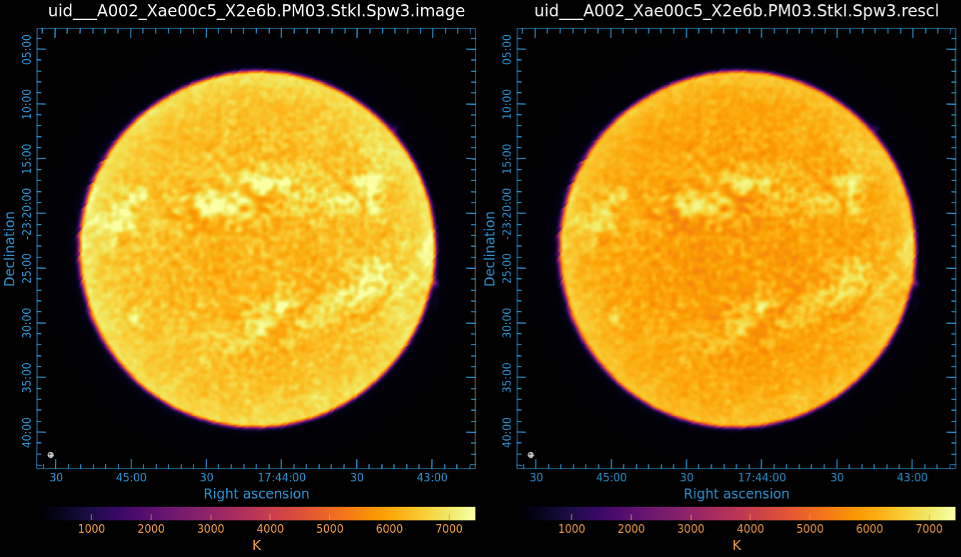
Copy the output URL into a browser to view your CARTA session. You can see the full-sun image as shown in Figure 1. Select and load:
uid___A002_Xae00c5_X2e6b.PM03.StkI.Spw3.image
Rescaling after Imaging
White et al. (2017) recommended that the standard ALMA single-dish image products be scaled to match their best determination of quiet-Sun temperatures at disk center:
- 5900K averaged over an 80" square region centered on the apparent disk center at Band6
- 7300K averaged over a 120" square region centered on the apparent disk center at Band3
- uncertainties of about 100K
For the re-scaling in Band6, the following immath command is executed.
#In CASA
res = imstat(sd_img+'.image', region='circle[[400pix,400pix],80pix]')

immath(imagename=sd_img+'.image', expr='IM0*'+str(5900./res['mean'][0]), outfile=sd_img+'.rescl')
When you image solar Band3 data, choose region='circle[[200pix,200pix],40pix]' and expr='IM0*'+str(7300./res['mean'][0]) instead.
Now append the following image in CARTA:
uid___A002_Xae00c5_X2e6b.PM03.StkI.Spw3.rescl
Note: All full-sun images that are included in the SV data package (ex. Sunspot_Band6_ReferenceImages.tgz) were not applied the re-scaling because the SV data were released before publishing White et al. (2017). When you use the full-sun image of the SV data for your studies, you should be done the re-scaling process. While the archive data obtained in Cycles were applied the re-scaling process.