Protoplanetary Disk Simulation - VLA-CASA6.4.1
Overview
The following tutorial shows how to adopt typical parameters for simulating Karl G. Jansky VLA data. We will use the same image as the ALMA tutorial Protoplanetary Disk Simulation. Follow this link to obtain the protoplanetary disk model image. Model images are in units of Jy/pixel. Other simulation options, e.g., using component lists, or how to use the toolkit are explained in the Simulations in CASA section of the CASAguides.
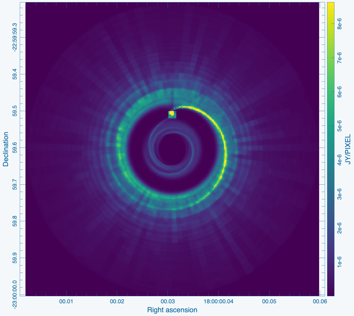
Figure 1 shows the model that we will use for this simulation tutorial.
 |
The ALMA version of the tutorial describes CASA tools to derive the center of the image. We will use their results and specify direction='J2000 18h00m00.031s -22d59m59.6s' for all of our simulations. The image center can also be determined with the CASA viewer. Given that the VLA primary beams at the VLA frequencies are much larger than the image, the precise pointing direction center is less important.
We will mostly use the simobserve and simanalyze tasks similar to the ALMA tutorials (we will follow the ALMA plotted image sequence). The ALMA model, however, has a specified frequency of 672GHz and we will adapt it to work for VLA frequencies.
Note that simobserve has a few limitations, e.g., it cannot simulate different spectral windows (spw). If this is desired, each spw needs to be simulated separately, followed by a concatenation (concat) of all simulated MeasurementSets (MS). In addition, simobserve has no option to add pointing errors to the simulated data. All VLA configurations and the VLA receiver temperatures are, however, accessible in simobserve.
Q-band, 128MHz bandwidth, noiseless image, 1hr integration time, A-configuration, no deconvolution
Let's start with a simulation at 44GHz (Q-band), with a bandwidth of 128MHz, the largest possible bandwidth of a spectral window at the VLA. We will simulate observations with the VLA A-configuration as it provides the resolution that is needed for the disk to be well resolved. To start with, we do not add any noise to the data.
# In CASA
simobserve(project='psimvla1',
                    skymodel='ppdisk672_GHz_50pc.fits',
                    inbright='3e-5Jy/pixel',
                    incenter='44GHz',
                    inwidth='128MHz' ,
                    setpointings=True,
                    integration='2s',
                    direction='J2000 18h00m00.031s -22d59m59.6s',
                    mapsize= '0.78arcsec',
                    obsmode='int',
                    antennalist='vla.a.cfg',
                    hourangle='transit',
                    totaltime='3600s',
                    thermalnoise='',
                    graphics='both',
                    overwrite=True)
project: The name of our project is psimvla1. All data will be stored in a directory that is created using the project name.
skymodel: The input model image in Jy/pixel units. We overwrite the fits header to assume that the model is valid for 44GHz using the incenter parameter and we set the bandwidth to 128MHz with inwidth. We also adjust the peak to a lower [math]\displaystyle{ 3\times10^{-5} }[/math]Jy/pixel value with the inbright parameter, an expected decline of flux at the the lower frequency tail of a dust black body distribution.
setpointings: allows simobserve to derive the pointing positions by its own algorithm. Given that the primary beam at Q-band is about 1 arcminute (see the VLA Observational Status Summary (OSS)), and the size of the model is less than an arcsecond, a single pointing will be adequate.
integration: To avoid time smearing, we follow the guidance for data rates in the VLA OSS and assume 2s correlator integration time per visibility.
direction: the center of the map. For a single pointing this is equivalent to the pointing center.
obsmode: int is used for interferometric data such as VLA observations.
antennalist: the VLA configuration antenna position file. The files are available in CASA via 'vla.x.cfg' where 'x' is the name of the array configuration. Here 'vla.a.cfg' is the VLA A-configuration (the python command os.getenv("CASAPATH").split()[0]+"/data/alma/simmos/" shows the directory that contains all array configurations that are packaged in CASA).
hourangle: is used to simulate observations at a specific hour angle. We use 'transit' for culmination.
totaltime: This is the time on source.
thermalnoise: We leave this parameter empty for this noise-less simulation.
graphics: 'both' will show graphics on the screen and save them as png files in the project directory.
overwrite: True will overwrite previous results; be careful when running multiple setups as the files may have different names and only the files with the same names will be overwritten.
The output of the simulation is shown in Figures 2 and 3. The first image is the sky coverage which shows clearly that the primary beam exceeds the size of the model image by far. The other outputs are explained in the caption of Figure 3.
 |
 |
The task simanalyze can now process the newly created MS and image the data:
# In CASA
simanalyze(project='psimvla1',
                    image=True,
                    vis='psimvla1.vla.a.ms',
                    imsize=[192, 192],
                    interactive=False,
                    niter=0,
                    weighting='briggs',
                    pbcor=False,
                    stokes='I',
                    analyze=True,
                    showuv=False,
                    showpsf=True,
                    showmodel=True,
                    showconvolved=True,
                    showclean=True,
                    showresidual=True,
                    showdifference=True,
                    showfidelity=True,
                    graphics='both',
                    overwrite=True)
project: The project (directory) name, same as in our call for simobserve.
image: True will image the visibilities with the following sub-parameters.
vis: The input MS inside the project directory. Note that simobserve's notation is to use the project name appended by the antenna configuration file name.
imsize: the number of pixels for the image dimensions. We use 192 for each axis. By default simobserve will use the pixel size of the model image as the cell size for each simulated image pixel (3.11 milli-arcseconds in our case).
interactive: If set to True, the cleaning will be interactive to allow the step by step setting of clean boxes and clean depths (see the VLA imaging topical guide). We will turn this feature off.
niter: number of clean iterations. We start with a dirty map and set niter=0.
weighting: (cf. Image weighting schemes). We will use briggs which defaults to a robust = 0.5.
pbcor: If set to True the image will be primary beam corrected. In our case of a very large primary beam (see Figure 1), primary beam correction will introduce very small corrections, so we turn it off.
stokes: the Stokes polarization to be calculated; we want Stokes I.
analyze: When set to True, simobserve will perform basic analysis of the generated images and create hard copies of the following displays.
showuv: We set this to False as we already show the uv-coverage in the simobserve output (see Figure 3).
showpsf: Whereas the 'natural' weighted psf is already shown in Figure 3, the psf here is calculated based on the specified 'briggs' weighting scheme (where the default robust subparameter is 0.5).
showconvolved: creates a plot of the model convolved with the synthesized clean beam.
showclean: shows the deconvolved image (in our case we do not perform deconvolution, but show the plot to be consistent with subsequent runs).
showresidual: a plot of the residual image after deconvolution.
showdifference: displays the difference between output cleaned image and input model sky image convolved with output clean beam, i.e., it shows remaining clean artefacts.
showfidelity: a fidelity image, as defined by [math]\displaystyle{ \frac{I}{|I-T|} }[/math] where [math]\displaystyle{ I }[/math] is the observed image and [math]\displaystyle{ T }[/math] the sky model, see the simanalyze CASAdoc help. Note that the fidelity image is unit-less, but a bug in simobserve still shows it as Jy/beam.
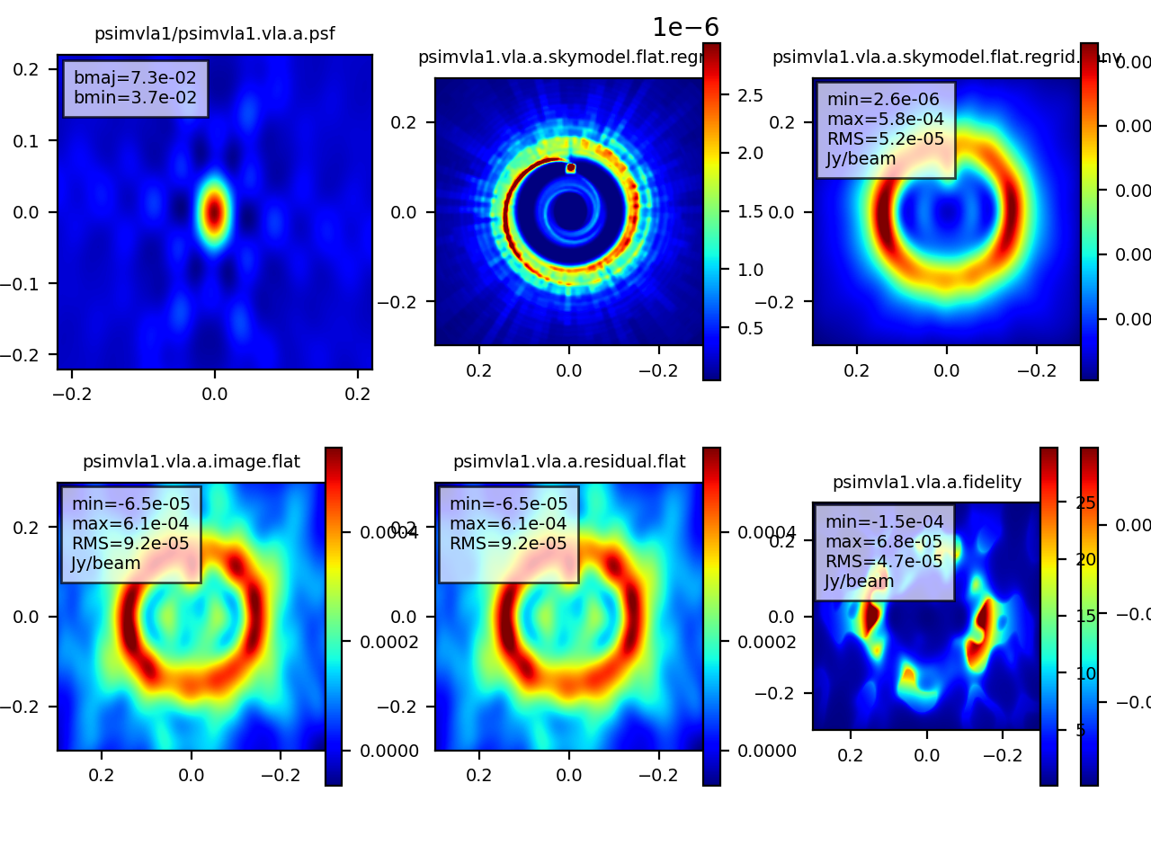
The resulting plots of our first simulation are shown in Figure 4 (only the last figure may be shown on the screen; all figures are in the simulation directory, here: psimvla1). Since this is a dirty image only (niter=0), the image and residual are the same dirty image. We also did not turn on any thermal noise and the image corruptions are all due to the incomplete uv-coverage of our simulation.
Q-band, 128MHz bandwidth, noiseless image, 1hr integration time, A-configuration, cleaned
As a second step we will deconvolve this dataset. This could be done inside the same project, but for a separation of our use cases, we will recreate the MS with simobserve and modify the simanalyze call.
# In CASA
simobserve(project='psimvla2', skymodel='ppdisk672_GHz_50pc.fits', inbright='3e-5Jy/pixel', incenter='44GHz', inwidth='128MHz' , setpointings=True, integration='2s',  direction='J2000 18h00m00.031s -22d59m59.6s',  mapsize= '0.78arcsec', obsmode='int', antennalist='vla.a.cfg', hourangle='transit', totaltime='3600s',  thermalnoise='', graphics='both', overwrite=True)

simanalyze(project='psimvla2', image=True, vis='psimvla2.vla.a.ms',  imsize=[192, 192], interactive=False, niter=1000, threshold='1e-4Jy', weighting='briggs',  pbcor=False, stokes='I', analyze=True, showuv=False, showpsf=True, showmodel=True, showconvolved=True, showclean=True, showresidual=True, showdifference=True, showfidelity=True, graphics='both', overwrite=True)
The only difference to the earlier call of simanalyze is our setting of niter=1000, threshold='1e-4Jy' which corresponds to a maximum number of 1000 clean iterations and a clean threshold of 0.1mJy. The threshold was chosen based on the previous image to be a few times above the rms of the image, and the niter is set large enough to reach the threshold. As expected, the residual image is now flatter and the bulk of the sidelobes disappear.
 |
Q-band, 128MHz bandwidth, noisy, 1hr integration time, A-configuration
We now add environmental effects using an opacity and a sky temperature. These values can be calculated through an atmospheric model based on weather parameters for the VLA site. The Analysis Utilities toolbox can perform the calculations using the au.estimateOpacity method. For good VLA conditions (pwv=4mm) we estimate a zenith opacity of 0.065 and a sky temperature of 20K at 44GHz. These values are supplied as tau0 and t_sky subparameters to thermalnoise='tsys-manual' in simobserve. The task, however, does not add phase noise due to pwv variations across the array. The sm.settrop tool can be used for the more sophisticated tropospheric models. A description is given in Corrupting Simulated Data. The EVLA receiver and antenna contributions to the noise are known to simobserve.
# In CASA
simobserve(project='psimvla3', skymodel='ppdisk672_GHz_50pc.fits', inbright='3e-5Jy/pixel', incenter='44GHz', inwidth='128MHz' , setpointings=True, integration='2s',  direction='J2000 18h00m00.031s -22d59m59.6s',  mapsize= '0.78arcsec', obsmode='int', antennalist='vla.a.cfg', hourangle='transit', totaltime='3600s',  thermalnoise='tsys-manual', tau0=0.065, t_sky=20, graphics='both', overwrite=True)
The simobserve output is identical to Figures 2 and 3 since we did not change any parameters that influence the figure. Now let's analyse the MS.
# In CASA
simanalyze(project='psimvla3', image=True, vis='psimvla3.vla.a.noisy.ms', imsize=[192, 192], interactive=False, niter=1000, threshold='1e-4Jy', weighting='briggs',  pbcor=False, stokes='I', analyze=True, showuv=False, showpsf=True, showmodel=True, showconvolved=True, showclean=True, showresidual=True, showdifference=True, showfidelity=True, graphics='both', overwrite=True)
The results are displayed in Figure 6. The noise is dominating the image as expected.
 |
Comparison with the VLA Exposure Calculator
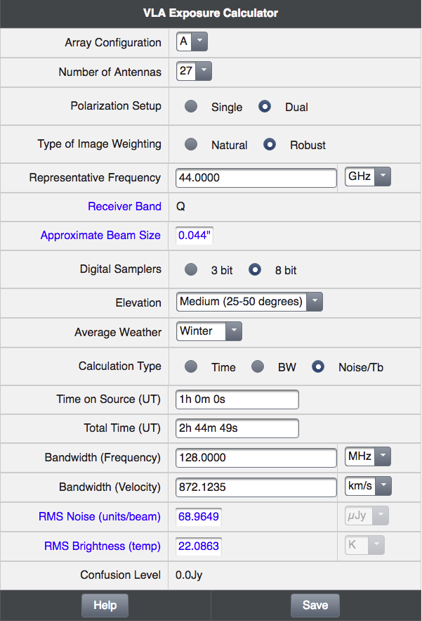
We can compare the simulation to the predicted VLA sensitivity via the VLA Exposure Calculator Tool (ECT). Using winter observing conditions (for good pwv), a medium elevation (see Figure 3), 128MHz bandwidth at a frequency of 44GHz, the ECT predicts a beam size of 0.044" and which is compatible to our simulations (see Figures 3 and 6). The ECT output is shown in Figure 7.
 |
The rms provided in Figure 6 is over the entire image and includes the source. It is therefore not representative to the thermal noise. To obtain a better noise figure, we now produce an image with the same parameters as simanalyze, but with a larger image size directly via tclean. Since the briggs parameter in simanalyze defaults to robust=0.5, we will use the same value here. The pblimit is a parameter used to define the value of the antenna primary beam gain, below which wide-field gridding algorithms such as 'mosaic' and 'awproject' will not apply normalization (and will therefore set to zero). For gridder='standard', there is no pb-based normalization during gridding and so the value of this parameter is ignored. The sign of the pblimit parameter, however, is used for a different purpose. If positive, it defines a T/F pixel mask that is attached to the output residual and restored images. If negative, this T/F pixel mask is not included. We will use pblimit=-0.1 here.
# In CASA
tclean(vis='psimvla3/psimvla3.vla.a.noisy.ms', imagename='psim3-bigimage', imsize=[640, 640], cell='3.11e-3arcsec',  specmode='mfs',  gridder= 'standard', deconvolver='hogbom', weighting='briggs', pblimit=-0.1, robust=0.5, niter=1000, threshold='1e-4Jy')
Open the image in the viewer:
# In CASA
viewer('psim3-bigimage.image')
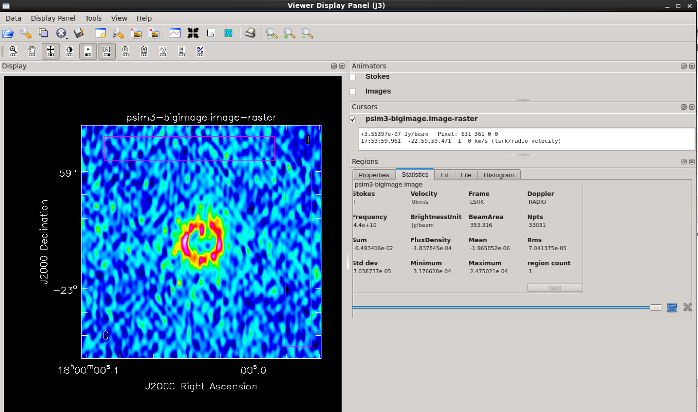
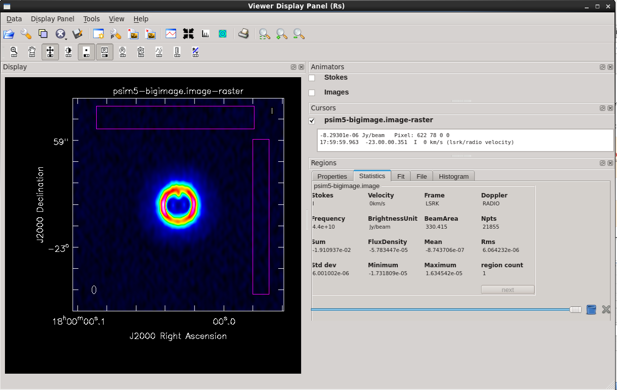
Measuring the noise statistics away from the source (Figure 8) gives a value of about 7e-5Jy/beam which is in very good agreement with the ECT predicted noise figure of 6.9e-5 Jy/beam.
 |
Q-band, 8GHz bandwidth, noisy, 1hr integration time, A-configuration
To achieve a better signal-to-noise ratio, we will now extend our bandwidth from 128MHz to 8GHz. The current implementation of simobserve has no channelization so the simulation will not have the better uv-coverage that is obtained in multi-frequency imaging. Consecutive simulations with different spws, and combined MSs, however, can achieve that and we will show how to obtain a multi-channel MS below. In addition, for large channel widths, one needs to be careful not to introduce bandwidth smearing. Our target is luckily near the phase center of the image and bandwidth smearing will be minimal.
# In CASA
simobserve(project='psimvla4',   skymodel='ppdisk672_GHz_50pc.fits', inbright='3e-5Jy/pixel', incenter='44GHz', inwidth='8GHz' , setpointings=True, integration='2s',  direction='J2000 18h00m00.031s -22d59m59.6s',  mapsize= '0.78arcsec', obsmode='int', antennalist='vla.a.cfg', hourangle='transit', totaltime='3600s',  thermalnoise='tsys-manual', tau0=0.065, t_sky=20, graphics='both', overwrite=True)
The simobserve output again is identical to Figure 3.
# In CASA
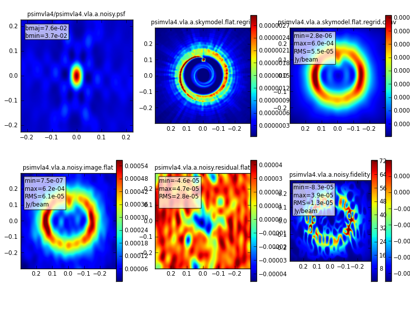
simanalyze(project='psimvla4', image=True, vis='psimvla4.vla.a.noisy.ms',  imsize=[192, 192], interactive=False, niter=10000, threshold='5e-5Jy', weighting='briggs',  pbcor=False, stokes='I', analyze=True, showuv=False, showpsf=True, showmodel=True, showconvolved=True, showclean=True, showresidual=True, showdifference=True, showfidelity=True, graphics='both', overwrite=True)
The image (see Figure 9) is clearly better defined, as expected from a broader bandwidth. We also decreased the cleaning threshold to 0.05mJy and added a few more iterations to reach this threshold.
 |
Multi-Term-Multi-Frequency Synthesis Imaging
In reality, the 8GHz bandwidth is not confined to a single channel but distributed across many channels. This results in a spread out uv-coverage as it depends on the projected baselines expressed in number of wavelengths, so channels are slightly displaced from each other. Therefore, combining the channels in a multi-frequency synthesis (mfs) does not only increase the sensitivity, but also the image fidelity through a better defined psf. Channelization and mfs imaging also reduce bandwidth smearing effects.
As mentioned above, simobserve naturally does not channelize the visibilities when the input image is not channelized. In the following, we will channelize the MS and, to produce a more realistic source, we will also apply a spectral index of [math]\displaystyle{ S\propto\nu^{-1.5} }[/math] at the same time.
To start with, we need to create a multi-channel model image. The following script converts our current model image from fits to the CASA image format with importfits. We then create 64 planes, apply the spectral index, and fix the headers accordingly to bring them into consecutive frequency order. Each channel is specified to a width of 128MHz (real VLA data would have typical channel widths of 2MHz). Finally, our individual planes are combined into a cube ppdisk-combined_spx.im with the ia.imageconcat tool method.
(Note that for some configurations copy and paste of more than a single command do not work. For those cases, start with %cpaste, then copy and paste all code lines, and finish with ---.)
# In CASA
importfits(fitsimage="ppdisk672_GHz_50pc.fits", imagename="ppdisk_Q_50pc.im")
stats=imstat(imagename='ppdisk_Q_50pc.im')
maximum=stats['max'][0]
ratio=3e-5/maximum
for x in range (0, 64):
     y=40+x*0.128
     immath(imagename="ppdisk_Q_50pc.im", mode='evalexpr', expr="IM0*"+str(ratio)+"*(("+str(y)+"/40)^-1.5)", outfile="ppdisk_Q_50pc_spx_"+str(x)+".im")
     imhead(imagename="ppdisk_Q_50pc_spx_"+str(x)+".im", mode="put", hdkey="crval4", hdvalue=str(y)+"GHz")
     imhead(imagename="ppdisk_Q_50pc_spx_"+str(x)+".im", mode="put", hdkey="cdelt4", hdvalue="128MHz")
comb=ia.imageconcat(outfile="ppdisk-combined_spx.im", infiles="ppdisk_Q_50pc_spx*.im",  axis=3, relax=True, tempclose=False, reorder=True, overwrite=True)
comb.close()
Using this model cube in simobserve will produce the channelized visibilities.
# In CASA
simobserve(project='psimvla4mfs',   skymodel='ppdisk-combined_spx.im',  setpointings=True, integration='2s',  direction='J2000 18h00m00.031s -22d59m59.6s',  mapsize= '0.78arcsec', obsmode='int', antennalist='vla.a.cfg', hourangle='transit', totaltime='3600s',  thermalnoise='tsys-manual', tau0=0.065, t_sky=20, graphics='none', overwrite=True)
simobserve and simanalyze assumes that, if the model is a cube, the output will be a cube too. In our case, however, we will produce a single multi-frequency synthesis continuum image so we have to use other, general CASA tasks for imaging and display.
Let's first have a look at the new uv-coverage. Each channel is displayed in a different color in Figure 10:
# In CASA
plotms(vis='psimvla4mfs/psimvla4mfs.vla.a.noisy.ms', xaxis='Uwave', yaxis='Vwave',coloraxis='channel')
 |
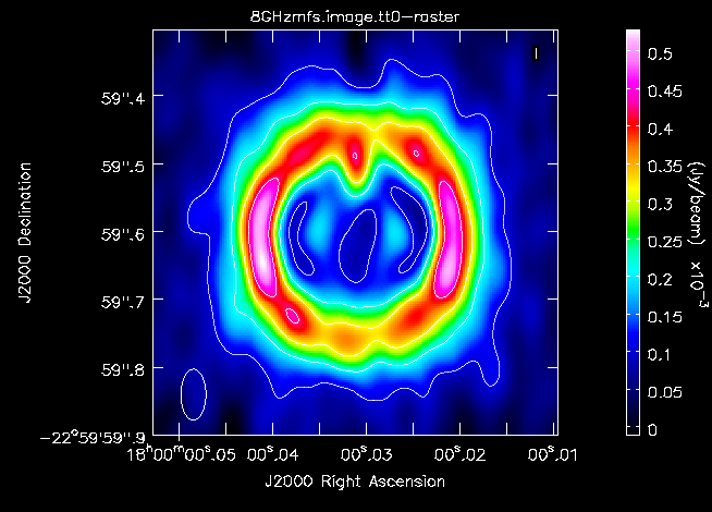
We will now create a continuum image with the mfs technique, and, to recover the spectral index, we will use the Multi-term Taylor expansion in frequency (mtmfs, see [1]). We will use nterms=2 to derive the spectral index. The spectral index map, however, is fairly sensitive to the scales in the image. A regular Hogbom clean based on point sources, typically creates maps with too steep spectral indices when applied to extended emission. To avoid this effect, we therefore use the multi-scale algorithm with a range of scales.
# In CASA
tclean(vis='psimvla4mfs/psimvla4mfs.vla.a.noisy.ms', imagename='psimvla4mfs/8GHzmfs', imsize=[192, 192], cell='3.11e-3arcsec', specmode='mfs', gridder='standard', deconvolver='mtmfs', nterms=2, scales=[0,2,4,8,13,20,40],  niter=1000, threshold='2e-4Jy', weighting='briggs', pblimit=-0.1, robust=0.5)
As before, we are not attempting primary beam corrections as the image is very small compared to the primary beam (see Figure 2).
The images can be displayed with the viewer. Figure 11 is 8GHzmfs.image.tt0 and Figure 12 is 8GHzmfs.alpha, both located under the directory psimvla4mfs. In Figure 12, we show the contours of the tt0 image on the tt0 image itself as well as on the spectral index map to check for the signal-to-noise at each position.
 |
 |
As seen in Figure 11, this method should produce a somewhat better fidelity than the non-mfs image shown in Figure 9, although a direct comparison is difficult given the spectral index that we introduced. The spectral index map itself (Figure 12), unfortunately, is dominated by noise, even at the brightest regions, partly due to the pwv that we assumed. This results in a relatively unreliable spectral index map overall, although the values scatter around the spectral index of -1.5 that we inserted earlier.
Q-band, 8GHz bandwidth, noisy, 4hr integration time, A-configuration
Let's improve the signal-to-noise ratio (and uv-coverage) of the observations even further by going to 4hr on-source integration, via totaltime='14400s' . Given that mfs imaging only marginally improved the image, for simplicity we will go back to using the original, unchannelized 8GHz bandwidth.
# In CASA
simobserve(project='psimvla5',   skymodel='ppdisk672_GHz_50pc.fits', inbright='3e-5Jy/pixel',  incenter='44GHz', inwidth='8GHz' , setpointings=True, integration='2s',  direction='J2000 18h00m00.031s -22d59m59.6s',  mapsize= '0.78arcsec', obsmode='int', antennalist='vla.a.cfg', hourangle='transit', totaltime='14400s',  thermalnoise='tsys-manual', tau0=0.065, t_sky=20, graphics='both', overwrite=True)
Figure 13 shows a better uv-coverage (lower left image) and the 4hr observation is also marked by a wider red bar in the top left image. This also improved the shape of the natural weighted psf.
 |
# In CASA
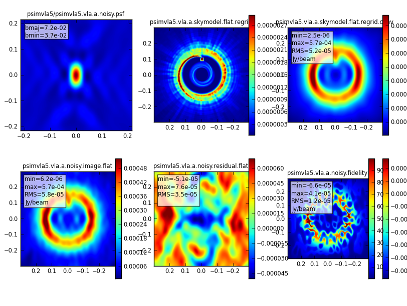
simanalyze(project='psimvla5', image=True, vis='psimvla5.vla.a.noisy.ms',  imsize=[192, 192], interactive=False, niter=1000, threshold='2e-5Jy', weighting='briggs',  pbcor=False, stokes='I', analyze=True, showuv=False, showpsf=True, showmodel=True, showconvolved=True, showclean=True, showresidual=True, showdifference=True, showfidelity=True, graphics='both', overwrite=True)
Given the expected deeper image, we reduced the cleaning threshold to 0.02mJy, and the result is shown in Figure 14. The image now is fairly close to the true sky model convolved with the clean beam.
 |
Comparison with the VLA Exposure Calculator
We compare again the simulation to the predicted VLA sensitivity via the VLA Exposure Calculator Tool (ETC). Using 8GHz bandwidth 4hr on-source, and a low elevation due to the longer observations, the ECT predicts a rms of ~7.1[math]\displaystyle{ \mu Jy }[/math] (see Figure 15):
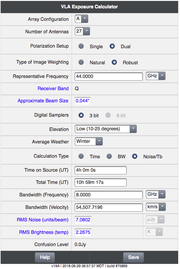 |
Using the same settings but a medium elevation results in ~5.4 [math]\displaystyle{ \mu Jy }[/math]. Note that the ECT switched to the 3-bit samplers to accommodate the large bandwidth. The simulator, however, assumes 8-bit samplers, which provide about 15% better sensitivity than the 3-bit samplers of the VLA. For a discussion, see the VLA Samplers page.
Similar to the case of 128MHz bandwidth 1hr case, we produce a larger image to be able to measure the image rms in a signal-free region.
# In CASA
tclean(vis='psimvla5/psimvla5.vla.a.noisy.ms', imagename='psim5-bigimage', imsize=[640, 640], cell='3.11e-3arcsec',  specmode='mfs',  gridder= 'standard', deconvolver='hogbom', weighting='briggs', pblimit=-0.1, robust=0.5, niter=10000, threshold='2e-5Jy')
Open the image in the viewer
# In CASA
viewer('psim5-bigimage.image')
Measuring the noise statistics away from the source (Figure 16), gives a value of about 6mJy/beam which is in very good agreement with the exposure calculator predictions between the two elevation settings.
 |
Q-band, 8GHz bandwidth, noisy, 1hr integration time, C-configuration
Our last Q-band simulation will use the same atmospheric conditions, but we will now simulate the observations with the VLA C-configuration (specified with the antennalist parameter).
# In CASA
simobserve(project='psimvla6',   skymodel='ppdisk672_GHz_50pc.fits', inbright='3e-5Jy/pixel',  incenter='44GHz', inwidth='8GHz' , setpointings=True, integration='2s',  direction='J2000 18h00m00.031s -22d59m59.6s',  mapsize= '0.78arcsec', obsmode='int', antennalist='vla.c.cfg', hourangle='transit', totaltime='3600s',  thermalnoise='tsys-manual', tau0=0.065, t_sky=20, graphics='both', overwrite=True)
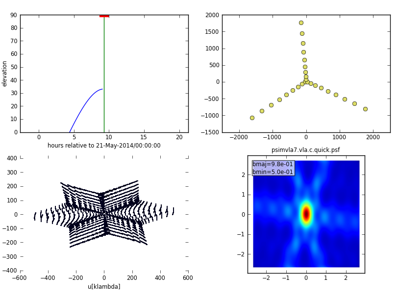
As expected, the extent of the uv-coverage decreases by a factor of about 10 (expressed in wavelengths) and the synthesized beam size increases by the same factor, as seen in Figure 17.
 |
Let's check the images:
# In CASA
simanalyze(project='psimvla6', image=True, vis='psimvla6.vla.c.noisy.ms',  imsize=[1728, 1728], interactive=False, niter=1000, threshold='1e-4Jy', weighting='briggs',  pbcor=False, stokes='I', analyze=True, showuv=False, showpsf=True, showmodel=True, showconvolved=True, showclean=True, showresidual=True, showdifference=True, showfidelity=True, graphics='both', overwrite=True)
Note that the output file names will now change and reflect C-configuration in their names. The resulting images are displayed in Figure 18, where the images now look like a point source with the degraded resolution. The surface brightness sensitivity of the observations, however, increases and we can clean to a lower threshold of 0.1mJy. simobserve automatically detected that the beam is massively oversampled and that a larger image size will provide a better field of view.
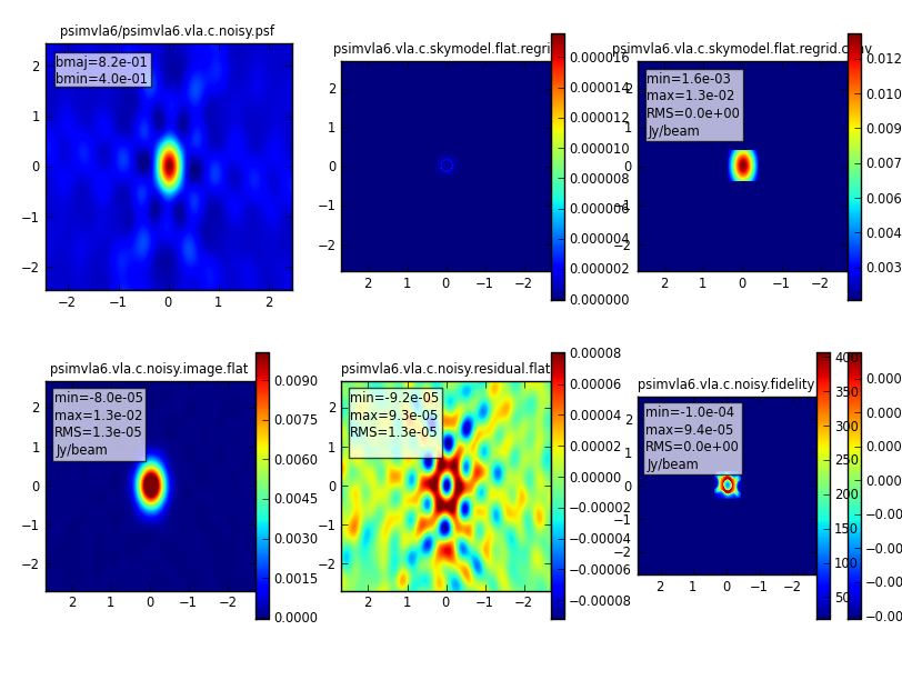 |
The sharp edges in some of the images show the boundaries of the original model image which has non-zero for all pixels. The increased field of view was simply padded with masked values.
To combine the data of two different array configurations, we refer to the VLA Data Combination Guide.
X-band, 4GHz bandwidth, noisy, 1hr integration time, A-configuration
Finally, we change the frequency and perform an X-band (10GHz), A-configuration simulation. Since X-band has a maximum bandwidth of 4GHz, we will reduce it to this value. We will also lower the flux density of the model to 0.01mJy given that the brightness of the model will likely be lower, too. The atmospheric conditions are as before, but note that X-band observations can be scheduled under worse conditions, which have less impact on the data quality at lower frequencies. (We also note a bug in simobserve which does not allow us to use t_sky values of <11 -- the correct value for X-band would be about 4K according to Analysis Utils).
# In CASA
simobserve(project='psimvla7',   skymodel='ppdisk672_GHz_50pc.fits', inbright='1e-5Jy/pixel',  incenter='10GHz', inwidth='4GHz' , setpointings=True, integration='2s',  direction='J2000 18h00m00.031s -22d59m59.6s',  mapsize= '0.78arcsec', obsmode='int', antennalist='vla.a.cfg', hourangle='transit', totaltime='3600s',  thermalnoise='tsys-manual', tau0=0.006, t_sky=11, graphics='both', overwrite=True)
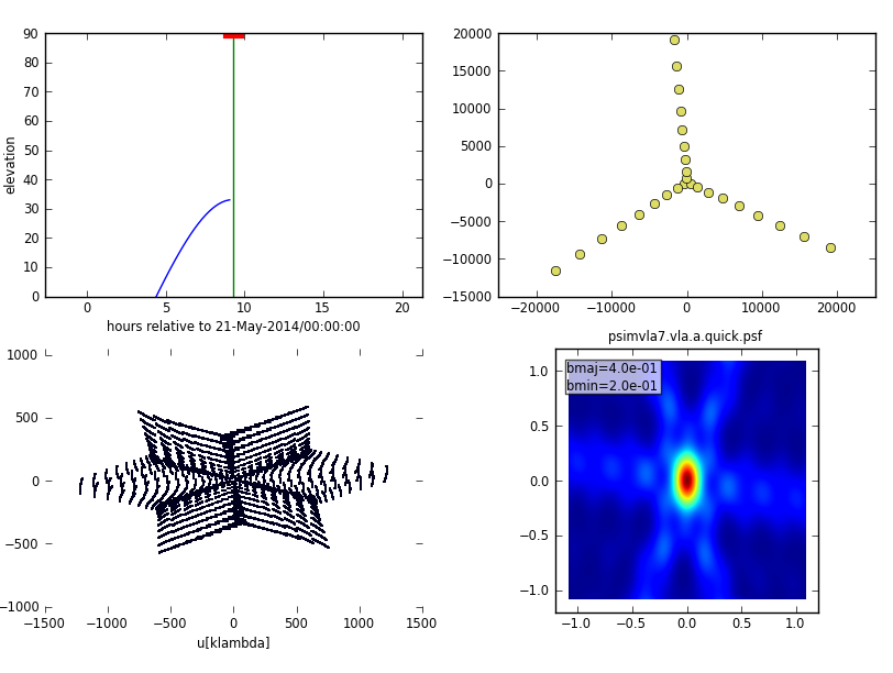
When expressed in wavelengths, the uv-coverage and synthesized beam are somewhere in between that of Q-band A-configuration and C-configuration as expected (Figure 19).
 |
# In CASA
simanalyze(project='psimvla7', image=True, vis='psimvla7.vla.a.noisy.ms',  imsize=[192, 192], interactive=False, niter=1000, threshold='3e-5Jy', weighting='briggs',  pbcor=False, stokes='I', analyze=True, showuv=False, showpsf=True, showmodel=True, showconvolved=True, showclean=True, showresidual=True, showdifference=True, showfidelity=True, graphics='both', overwrite=True)
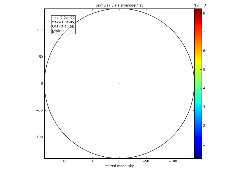
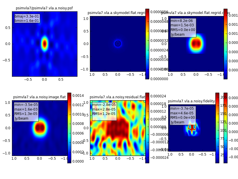
The larger primary beam of the X-band data is shown in Figure 20, where the model image is barely visible in the center. The simulated images are shown in Figure 21. The ring shape is still visible in the results although it is quite blurred given the larger beam. We note that the noise is considerably lower as expected from the lower band noise properties of the receiver and atmosphere. We adjusted the clean threshold accordingly. Again, simanalyze was overriding the image size as the psf would not have been adequately covered for the lower frequency.
 |
 |
Last checked on CASA Version 6.4.1
