First Look at Image Analysis CASA 6
This guide is written for CASA 6.1 and uses Python 3. The same functionality in implemented in Python 2 using CASA 5.7 at First Look at Image Analysis
The first few tutorials provided us with a spectral line data cube and a continuum image. Next we'd like to understand some of the properties of the images that we have produced.
In case you don't have the images from the first tutorials handy, let's start by copying the image files from the working_data directory to our current directory:
# In CASA
os.system("rm -rf sis14_twhya_cont.image")
os.system("cp -r ../working/sis14_twhya_cont.image .")
os.system("rm -rf twhya_n2hp.image")
os.system("cp -r ../working/twhya_n2hp.image .")
Recall that we orient ourselves with measurement sets (UV data) using the listobs task. For images, an analogous way to get basic header information is to use the imhead task.
# In CASA
imhead("sis14_twhya_cont.image")
imhead("twhya_n2hp.image")
CASA prints the image header information to the logger:
imhead	##########################################
imhead	##### Begin Task: imhead             #####
imhead	imhead(imagename="sis14_twhya_cont.image",mode="summary",hdkey="",hdvalue="",verbose=False)
ImageMetaData
ImageMetaData	Image name       : sis14_twhya_cont.image
ImageMetaData	Object name      : TW Hya
ImageMetaData	Image type       : PagedImage
ImageMetaData	Image quantity   : Intensity
ImageMetaData	Pixel mask(s)    : None
ImageMetaData	Region(s)        : None
ImageMetaData	Image units      : Jy/beam
ImageMetaData	Restoring Beam   : 0.789582 arcsec, 0.551785 arcsec, -58.4646 deg
ImageMetaData
ImageMetaData	Direction reference : J2000
ImageMetaData	Spectral  reference : LSRK (-> TOPO)
ImageMetaData	Velocity  type      : RADIO
ImageMetaData	Rest frequency      : 3.72637e+11 Hz
ImageMetaData	Pointing center     :  11:01:51.796000  -34.42.17.366000
ImageMetaData	Telescope           : ALMA
ImageMetaData	Observer            : cqi
ImageMetaData	Date observation    : 2012/11/19/07:37:00
ImageMetaData	Telescope position: [2.22506e+06m, -5.44006e+06m, -2.48168e+06m] (ITRF)
ImageMetaData
ImageMetaData	Axis Coord Type      Name             Proj Shape Tile   Coord value at pixel        Coord incr Units
ImageMetaData	----------------------------------------------------------------------------------------------------
ImageMetaData	0    0     Direction Right Ascension   SIN   256  256  11:01:51.796   128.00     -1.000000e-01 arcsec
ImageMetaData	1    0     Direction Declination       SIN   256  256 -34.42.17.366   128.00      1.000000e-01 arcsec
ImageMetaData	2    1     Stokes    Stokes                    1    1             I
ImageMetaData	3    2     Spectral  Frequency                 1    1   3.72637e+11     0.00 2.35055441345e+08 Hz
ImageMetaData	                     Velocity                                     0     0.00     -1.891126e+02 km/s
imhead	##### End Task: imhead               #####
imhead	##########################################

imhead	##########################################
imhead	##### Begin Task: imhead             #####
imhead	imhead(imagename="sis14_twhya_n2hp.image",mode="summary",hdkey="",hdvalue="",verbose=False)
ImageMetaData
ImageMetaData	Image name       : sis14_twhya_n2hp.image
ImageMetaData	Object name      : TW Hya
ImageMetaData	Image type       : PagedImage
ImageMetaData	Image quantity   : Intensity
ImageMetaData	Pixel mask(s)    : mask0
ImageMetaData	Region(s)        : None
ImageMetaData	Image units      : Jy/beam
ImageMetaData	Restoring Beam   : 0.709488 arcsec, 0.469052 arcsec, -53.779 deg
ImageMetaData
ImageMetaData	Direction reference : J2000
ImageMetaData	Spectral  reference : LSRK
ImageMetaData	Velocity  type      : RADIO
ImageMetaData	Rest frequency      : 3.72672e+11 Hz
ImageMetaData	Pointing center     :  11:01:51.796000  -34.42.17.366000
ImageMetaData	Telescope           : ALMA
ImageMetaData	Observer            : cqi
ImageMetaData	Date observation    : 2012/11/19/07:56:27
ImageMetaData	Telescope position: [2.22506e+06m, -5.44006e+06m, -2.48168e+06m] (ITRF)
ImageMetaData
ImageMetaData	Axis Coord Type      Name             Proj Shape Tile   Coord value at pixel      Coord incr Units
ImageMetaData	--------------------------------------------------------------------------------------------------
ImageMetaData	0    0     Direction Right Ascension   SIN   250  125  11:01:51.796   125.00   -8.000000e-02 arcsec
ImageMetaData	1    0     Direction Declination       SIN   250   50 -34.42.17.366   125.00    8.000000e-02 arcsec
ImageMetaData	2    1     Stokes    Stokes                    1    1             I
ImageMetaData	3    2     Spectral  Frequency                15    5   3.72672e+11     0.00 -6.21550826e+05 Hz
ImageMetaData	                     Velocity                                     0     0.00    5.000000e-01 km/s
imhead	##### End Task: imhead               #####
imhead	##########################################
Statistics
Often we'd like to measure basic image statistics and fluxes. Recall you can do these operations pretty easily in the viewer, by dragging out a box and then right-double clicking inside it to get statistics for that region. You can also get statistics using the imstat task.
# In CASA
my_stats = imstat("twhya_n2hp.image", chans="0~4")
The imstat task returns a python dictionary, and you can examine the contents as follows:
# In CASA
print(my_stats)
print(my_stats['rms'])
It's useful to see that the RMS is about 20 mJy/beam in the line cube.
You can also just print the dictionary to the terminal screen:
# In CASA
imstat("twhya_n2hp.image", chans="0~4")
This task is useful for measuring basic source characteristics. For example, calculate the statistics for a box encompassing the disk - you see that the integrated flux is about 1.5 Jy.
# In CASA
imstat("sis14_twhya_cont.image", box="100,100,150,150")
my_stats = imstat("sis14_twhya_cont.image", box="100,100,150,150")
print(my_stats['flux'])
Alternatively, a box defined off the disk will give image noise statistics.
# In CASA
imstat("sis14_twhya_cont.image", box="25,150,225,200")
Moments
For the spectral line cube, it's very useful to "collapse" the cube in various ways to analyze the emission. The immoments task lets you do this.
The first few "moments" are defined as follows:
 moments = -1 : mean value of the spectral coordinate
 moments =  0 : integrated value of the spectral coordinate
 moments =  1 : intensity weighted coordinate; traditionally used to get 'velocity fields'
 moments =  2 : intensity weighted dispersion of the coordinate; traditionally used to get "velocity dispersion"
A more complete description of image moments is given here in the CASA reference manual.
<figure id="Imaging-tutorial-analysis-mom0.png">

</figure>
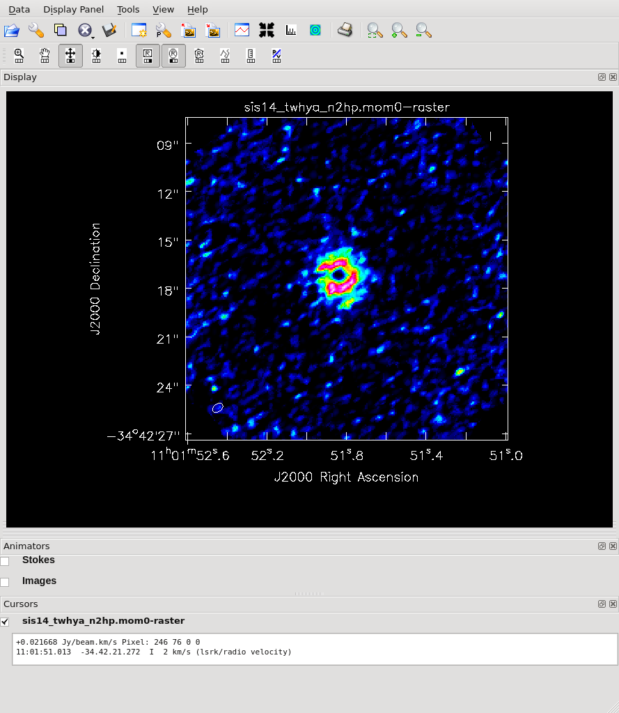
Let's make a moment 0 image clipped at ~1 sigma:
# In CASA
os.system("rm -rf sis14_twhya_n2hp.mom0")
immoments("twhya_n2hp.image",
          outfile="sis14_twhya_n2hp.mom0",
          includepix=[20e-3,100],
          chans="4~12",
          moments=0)
Make a moment 1 image clipped at ~2 sigma:
# In CASA
os.system("rm -rf sis14_twhya_n2hp.mom1")
immoments("twhya_n2hp.image",
          outfile="sis14_twhya_n2hp.mom1",
          includepix=[40e-3,100],
          chans="4~12",
          moments=1)
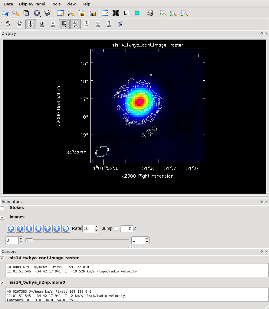
At this point we have a few really neat things to see: first the line shows a hole in the middle. Overlay it on the dust (continuum) disk using the viewer and you can notice that they align but with the N2H+ existing only outside a certain radius - in this case the "snow line". Also have a look at the velocity field to see the rotation of the disk.
The imview task has some command-line scripting capability. For example, here we show how to overlay the line moment 0 (as a contour plot) on the continuum.
<figure id="Imaging-tutorial-analysis-overlay.png">

</figure>
# In CASA
imview(raster={'file': 'sis14_twhya_cont.image',
'range': [-0.01,0.5]},
contour={'file': 'sis14_twhya_n2hp.mom0',
'levels': [0.5,0.6,0.7,0.8] })
Here, we are not using the primary beam corrected images and cubes when creating our moment maps. Remember that it's often very convenient to work in images before primary beam correction because the noise is the same across the field (e.g., this is a clean data set to search for signal) but it's very important to remember to apply this correction before calculating fluxes or intensities for science.
Export FITS images
CASA is great (of course) but you will ultimately want to export your data to a common format to analyze in other programs, share with other astronomers, or archive. It's easy to export images from CASA's image format to FITS images via the exportfits command.
# In CASA
exportfits(imagename="sis14_twhya_cont.image",
           fitsimage="twhya_cont.fits",
           overwrite=True)
For the cube we want to specify additionally that the frequency axis will be written out as velocity.
# In CASA
exportfits(imagename="twhya_n2hp.image",
           fitsimage="twhya_n2hp.fits",
           velocity=True,
           overwrite=True)