EVLA Continuum Tutorial 3C391
Overview
This article describes the calibration and imaging of a multiple-pointing EVLA continuum dataset on the supernova remnant 3C 391. The data were taken in OSRO1 mode, with 128 MHz of bandwidth in each of two widely spaced spectral windows, centered at 4.6 and 7.5 GHz, and were set up for full polarization calibration. To generate the full data reduction script described here, use the script extractor.
Getting hold of your data
The data are publicly available from the NRAO archive, under Project name TDEM0001. The archive lists two separate files; one taken on 2010-Apr-15, and the other on 2010-Apr-24. You will want to download the second file (file size 39.79 GB). This file contains data at the full 1-s time resolution.
Loading in your data
importevla(asdm='TDEM0001_sb1218006_1.55310.33439732639',vis='3c391_mosaic_fullres.ms',flagzero=True,shadow=True)
Examining your data
Before starting the calibration process, we want to get some basic information about the data set. To examine the observing conditions during the observing run, and to find out any known problems with the data, download the observer log. Simply fill in the known observing date (in our case 2010-Apr-24) as both the Start and Stop date, and click on the "Show Logs" button. The relevant log is labeled with the project code, TDEM0001, and can be downloaded as a PDF file.
To get a listing of the individual scans comprising the observation, the frequency setup, source list, and antenna locations, use the task listobs.
listobs(vis='3c391_ctm_mosaic_10s.ms',verbose=T)
listobs should now produce the following output in the casa logger:
2010-04-27 19:16:49	INFO	listobs::::casa	##########################################
2010-04-27 19:16:49	INFO	listobs::::casa	##### Begin Task: listobs            #####
2010-04-27 19:16:49	INFO	listobs::::casa
2010-04-27 19:16:49	INFO	listobs::ms::summary	================================================================================
2010-04-27 19:16:49	INFO	listobs::ms::summary+	           MeasurementSet Name:  /export/home/hamal/jmiller/TDEM0001_sb1218006/3c391_mosaic_fullres.ms      MS Version 2
2010-04-27 19:16:49	INFO	listobs::ms::summary+	================================================================================
2010-04-27 19:16:49	INFO	listobs::ms::summary+	   Observer: Dr. James Miller-Jones     Project: T.B.D.
2010-04-27 19:16:49	INFO	listobs::ms::summary+	Observation: EVLA
2010-04-27 19:16:49	INFO	listobs::ms::summary	Data records: 18666050       Total integration time = 28716 seconds
2010-04-27 19:16:49	INFO	listobs::ms::summary+	   Observed from   24-Apr-2010/08:01:34.5   to   24-Apr-2010/16:00:10.5 (UTC)
2010-04-27 19:17:47	INFO	listobs::ms::summary
2010-04-27 19:17:47	INFO	listobs::ms::summary+	   ObservationID = 0         ArrayID = 0
2010-04-27 19:17:47	INFO	listobs::ms::summary+	  Date        Timerange (UTC)          Scan  FldId FieldName    nVis   Int(s)   SpwIds
2010-04-27 19:17:47	INFO	listobs::ms::summary+	  24-Apr-2010/08:01:34.5 - 08:02:28.5     1      0 J1331+3030   35750  1        [0, 1]
2010-04-27 19:17:47	INFO	listobs::ms::summary+	              08:02:29.5 - 08:09:27.5     2      0 J1331+3030   272350 1        [0, 1]
2010-04-27 19:17:47	INFO	listobs::ms::summary+	              08:09:28.5 - 08:16:26.5     3      0 J1331+3030   272350 1        [0, 1]
2010-04-27 19:17:47	INFO	listobs::ms::summary+	              08:16:27.5 - 08:24:25.5     4      1 J1822-0938   311350 1        [0, 1]
2010-04-27 19:17:47	INFO	listobs::ms::summary+	              08:24:26.5 - 08:29:44.5     5      2 3C391 C1     207350 1        [0, 1]
2010-04-27 19:17:47	INFO	listobs::ms::summary+	              08:29:45.5 - 08:34:43.5     6      3 3C391 C2     194350 1        [0, 1]
2010-04-27 19:17:47	INFO	listobs::ms::summary+	              08:34:44.5 - 08:39:42.5     7      4 3C391 C3     194350 1        [0, 1]
2010-04-27 19:17:47	INFO	listobs::ms::summary+	              08:39:43.5 - 08:44:41.5     8      5 3C391 C4     194350 1        [0, 1]
2010-04-27 19:17:47	INFO	listobs::ms::summary+	              08:44:42.5 - 08:49:40.5     9      6 3C391 C5     194350 1        [0, 1]
2010-04-27 19:17:47	INFO	listobs::ms::summary+	              08:49:41.5 - 08:54:40.5    10      7 3C391 C6     195000 1        [0, 1]
2010-04-27 19:17:47	INFO	listobs::ms::summary+	              08:54:41.5 - 08:59:39.5    11      8 3C391 C7     194350 1        [0, 1]
2010-04-27 19:17:47	INFO	listobs::ms::summary+	              08:59:40.5 - 09:01:29.5    12      1 J1822-0938   71500  1        [0, 1]
2010-04-27 19:17:47	INFO	listobs::ms::summary+	              09:01:30.5 - 09:06:48.5    13      2 3C391 C1     207350 1        [0, 1]
2010-04-27 19:17:47	INFO	listobs::ms::summary+	              09:06:49.5 - 09:11:47.5    14      3 3C391 C2     194350 1        [0, 1]
2010-04-27 19:17:47	INFO	listobs::ms::summary+	              09:11:48.5 - 09:16:46.5    15      4 3C391 C3     194350 1        [0, 1]
2010-04-27 19:17:47	INFO	listobs::ms::summary+	              09:16:47.5 - 09:21:45.5    16      5 3C391 C4     194350 1        [0, 1]
2010-04-27 19:17:47	INFO	listobs::ms::summary+	              09:21:46.5 - 09:26:44.5    17      6 3C391 C5     194350 1        [0, 1]
2010-04-27 19:17:47	INFO	listobs::ms::summary+	              09:26:45.5 - 09:31:44.5    18      7 3C391 C6     195000 1        [0, 1]
2010-04-27 19:17:47	INFO	listobs::ms::summary+	              09:31:45.5 - 09:36:43.5    19      8 3C391 C7     194350 1        [0, 1]
2010-04-27 19:17:47	INFO	listobs::ms::summary+	              09:36:44.5 - 09:38:32.5    20      1 J1822-0938   70850  1        [0, 1]
2010-04-27 19:17:47	INFO	listobs::ms::summary+	              09:38:33.5 - 09:43:52.5    21      2 3C391 C1     208000 1        [0, 1]
2010-04-27 19:17:47	INFO	listobs::ms::summary+	              09:43:53.5 - 09:48:51.5    22      3 3C391 C2     194350 1        [0, 1]
2010-04-27 19:17:47	INFO	listobs::ms::summary+	              09:48:52.5 - 09:53:50.5    23      4 3C391 C3     194350 1        [0, 1]
2010-04-27 19:17:47	INFO	listobs::ms::summary+	              09:53:51.5 - 09:58:49.5    24      5 3C391 C4     194350 1        [0, 1]
2010-04-27 19:17:47	INFO	listobs::ms::summary+	              09:58:50.5 - 10:03:48.5    25      6 3C391 C5     194350 1        [0, 1]
2010-04-27 19:17:47	INFO	listobs::ms::summary+	              10:03:49.5 - 10:08:47.5    26      7 3C391 C6     194350 1        [0, 1]
2010-04-27 19:17:47	INFO	listobs::ms::summary+	              10:08:48.5 - 10:13:47.5    27      8 3C391 C7     195000 1        [0, 1]
2010-04-27 19:17:47	INFO	listobs::ms::summary+	              10:13:48.5 - 10:15:36.5    28      1 J1822-0938   70850  1        [0, 1]
2010-04-27 19:17:47	INFO	listobs::ms::summary+	              10:15:37.5 - 10:20:55.5    29      2 3C391 C1     207350 1        [0, 1]
2010-04-27 19:17:47	INFO	listobs::ms::summary+	              10:20:56.5 - 10:25:55.5    30      3 3C391 C2     195000 1        [0, 1]
2010-04-27 19:17:47	INFO	listobs::ms::summary+	              10:25:56.5 - 10:30:54.5    31      4 3C391 C3     194350 1        [0, 1]
2010-04-27 19:17:47	INFO	listobs::ms::summary+	              10:30:55.5 - 10:35:53.5    32      5 3C391 C4     194350 1        [0, 1]
2010-04-27 19:17:47	INFO	listobs::ms::summary+	              10:35:54.5 - 10:40:52.5    33      6 3C391 C5     194350 1        [0, 1]
2010-04-27 19:17:47	INFO	listobs::ms::summary+	              10:40:53.5 - 10:45:51.5    34      7 3C391 C6     194350 1        [0, 1]
2010-04-27 19:17:47	INFO	listobs::ms::summary+	              10:45:52.5 - 10:50:51.5    35      8 3C391 C7     195000 1        [0, 1]
2010-04-27 19:17:47	INFO	listobs::ms::summary+	              10:50:52.5 - 10:52:40.5    36      1 J1822-0938   70850  1        [0, 1]
2010-04-27 19:17:47	INFO	listobs::ms::summary+	              10:52:41.5 - 10:57:39.5    37      0 J1331+3030   194350 1        [0, 1]
2010-04-27 19:17:47	INFO	listobs::ms::summary+	              10:57:40.5 - 11:02:39.5    38      1 J1822-0938   195000 1        [0, 1]
2010-04-27 19:17:47	INFO	listobs::ms::summary+	              11:02:40.5 - 11:07:58.5    39      2 3C391 C1     207350 1        [0, 1]
2010-04-27 19:17:47	INFO	listobs::ms::summary+	              11:07:59.5 - 11:12:47.5    40      3 3C391 C2     187850 1        [0, 1]
2010-04-27 19:17:47	INFO	listobs::ms::summary+	              11:12:48.5 - 11:17:36.5    41      4 3C391 C3     187850 1        [0, 1]
2010-04-27 19:17:47	INFO	listobs::ms::summary+	              11:17:37.5 - 11:22:25.5    42      5 3C391 C4     187850 1        [0, 1]
2010-04-27 19:17:47	INFO	listobs::ms::summary+	              11:22:26.5 - 11:27:15.5    43      6 3C391 C5     188500 1        [0, 1]
2010-04-27 19:17:47	INFO	listobs::ms::summary+	              11:27:16.5 - 11:32:04.5    44      7 3C391 C6     187850 1        [0, 1]
2010-04-27 19:17:47	INFO	listobs::ms::summary+	              11:32:05.5 - 11:36:53.5    45      8 3C391 C7     187850 1        [0, 1]
2010-04-27 19:17:47	INFO	listobs::ms::summary+	              11:36:54.5 - 11:38:43.5    46      1 J1822-0938   71500  1        [0, 1]
2010-04-27 19:17:47	INFO	listobs::ms::summary+	              11:38:44.5 - 11:44:02.5    47      2 3C391 C1     207350 1        [0, 1]
2010-04-27 19:17:47	INFO	listobs::ms::summary+	              11:44:03.5 - 11:48:51.5    48      3 3C391 C2     187850 1        [0, 1]
2010-04-27 19:17:47	INFO	listobs::ms::summary+	              11:48:52.5 - 11:53:40.5    49      4 3C391 C3     187850 1        [0, 1]
2010-04-27 19:17:47	INFO	listobs::ms::summary+	              11:53:41.5 - 11:58:29.5    50      5 3C391 C4     187850 1        [0, 1]
2010-04-27 19:17:47	INFO	listobs::ms::summary+	              11:58:30.5 - 12:03:19.5    51      6 3C391 C5     188500 1        [0, 1]
2010-04-27 19:17:47	INFO	listobs::ms::summary+	              12:03:20.5 - 12:08:08.5    52      7 3C391 C6     187850 1        [0, 1]
2010-04-27 19:17:47	INFO	listobs::ms::summary+	              12:08:09.5 - 12:12:57.5    53      8 3C391 C7     187850 1        [0, 1]
2010-04-27 19:17:47	INFO	listobs::ms::summary+	              12:12:58.5 - 12:14:47.5    54      1 J1822-0938   71500  1        [0, 1]
2010-04-27 19:17:47	INFO	listobs::ms::summary+	              12:14:48.5 - 12:20:06.5    55      2 3C391 C1     207350 1        [0, 1]
2010-04-27 19:17:47	INFO	listobs::ms::summary+	              12:20:07.5 - 12:24:55.5    56      3 3C391 C2     187850 1        [0, 1]
2010-04-27 19:17:47	INFO	listobs::ms::summary+	              12:24:56.5 - 12:29:44.5    57      4 3C391 C3     187850 1        [0, 1]
2010-04-27 19:17:47	INFO	listobs::ms::summary+	              12:29:45.5 - 12:34:34.5    58      5 3C391 C4     188500 1        [0, 1]
2010-04-27 19:17:47	INFO	listobs::ms::summary+	              12:34:35.5 - 12:39:23.5    59      6 3C391 C5     187850 1        [0, 1]
2010-04-27 19:17:47	INFO	listobs::ms::summary+	              12:39:24.5 - 12:44:12.5    60      7 3C391 C6     187850 1        [0, 1]
2010-04-27 19:17:47	INFO	listobs::ms::summary+	              12:44:13.5 - 12:49:01.5    61      8 3C391 C7     187850 1        [0, 1]
2010-04-27 19:17:47	INFO	listobs::ms::summary+	              12:49:02.5 - 12:50:51.5    62      1 J1822-0938   71500  1        [0, 1]
2010-04-27 19:17:47	INFO	listobs::ms::summary+	              12:50:52.5 - 12:56:10.5    63      2 3C391 C1     207350 1        [0, 1]
2010-04-27 19:17:47	INFO	listobs::ms::summary+	              12:56:11.5 - 13:00:59.5    64      3 3C391 C2     187850 1        [0, 1]
2010-04-27 19:17:47	INFO	listobs::ms::summary+	              13:01:00.5 - 13:05:48.5    65      4 3C391 C3     187850 1        [0, 1]
2010-04-27 19:17:47	INFO	listobs::ms::summary+	              13:05:49.5 - 13:10:38.5    66      5 3C391 C4     188500 1        [0, 1]
2010-04-27 19:17:47	INFO	listobs::ms::summary+	              13:10:39.5 - 13:15:27.5    67      6 3C391 C5     187850 1        [0, 1]
2010-04-27 19:17:47	INFO	listobs::ms::summary+	              13:15:28.5 - 13:20:16.5    68      7 3C391 C6     187850 1        [0, 1]
2010-04-27 19:17:47	INFO	listobs::ms::summary+	              13:20:17.5 - 13:25:05.5    69      8 3C391 C7     187850 1        [0, 1]
2010-04-27 19:17:47	INFO	listobs::ms::summary+	              13:25:06.5 - 13:26:55.5    70      1 J1822-0938   71500  1        [0, 1]
2010-04-27 19:17:47	INFO	listobs::ms::summary+	              13:26:56.5 - 13:32:14.5    71      2 3C391 C1     207350 1        [0, 1]
2010-04-27 19:17:47	INFO	listobs::ms::summary+	              13:32:15.5 - 13:37:03.5    72      3 3C391 C2     187850 1        [0, 1]
2010-04-27 19:17:47	INFO	listobs::ms::summary+	              13:37:04.5 - 13:41:52.5    73      4 3C391 C3     187850 1        [0, 1]
2010-04-27 19:17:47	INFO	listobs::ms::summary+	              13:41:53.5 - 13:46:42.5    74      5 3C391 C4     188500 1        [0, 1]
2010-04-27 19:17:47	INFO	listobs::ms::summary+	              13:46:43.5 - 13:51:31.5    75      6 3C391 C5     187850 1        [0, 1]
2010-04-27 19:17:47	INFO	listobs::ms::summary+	              13:51:32.5 - 13:56:20.5    76      7 3C391 C6     187850 1        [0, 1]
2010-04-27 19:17:47	INFO	listobs::ms::summary+	              13:56:21.5 - 14:01:09.5    77      8 3C391 C7     187850 1        [0, 1]
2010-04-27 19:17:47	INFO	listobs::ms::summary+	              14:01:10.5 - 14:02:59.5    78      1 J1822-0938   71500  1        [0, 1]
2010-04-27 19:17:47	INFO	listobs::ms::summary+	              14:03:00.5 - 14:08:18.5    79      2 3C391 C1     207350 1        [0, 1]
2010-04-27 19:17:47	INFO	listobs::ms::summary+	              14:08:19.5 - 14:13:07.5    80      3 3C391 C2     187850 1        [0, 1]
2010-04-27 19:17:47	INFO	listobs::ms::summary+	              14:13:08.5 - 14:17:57.5    81      4 3C391 C3     188500 1        [0, 1]
2010-04-27 19:17:47	INFO	listobs::ms::summary+	              14:17:58.5 - 14:22:46.5    82      5 3C391 C4     187850 1        [0, 1]
2010-04-27 19:17:47	INFO	listobs::ms::summary+	              14:22:47.5 - 14:27:35.5    83      6 3C391 C5     187850 1        [0, 1]
2010-04-27 19:17:47	INFO	listobs::ms::summary+	              14:27:36.5 - 14:32:24.5    84      7 3C391 C6     187850 1        [0, 1]
2010-04-27 19:17:47	INFO	listobs::ms::summary+	              14:32:25.5 - 14:37:13.5    85      8 3C391 C7     187850 1        [0, 1]
2010-04-27 19:17:47	INFO	listobs::ms::summary+	              14:37:14.5 - 14:39:03.5    86      1 J1822-0938   71500  1        [0, 1]
2010-04-27 19:17:47	INFO	listobs::ms::summary+	              14:39:04.5 - 14:44:22.5    87      2 3C391 C1     207350 1        [0, 1]
2010-04-27 19:17:47	INFO	listobs::ms::summary+	              14:44:23.5 - 14:49:11.5    88      3 3C391 C2     187850 1        [0, 1]
2010-04-27 19:17:47	INFO	listobs::ms::summary+	              14:49:12.5 - 14:54:01.5    89      4 3C391 C3     188500 1        [0, 1]
2010-04-27 19:17:47	INFO	listobs::ms::summary+	              14:54:02.5 - 14:58:50.5    90      5 3C391 C4     187850 1        [0, 1]
2010-04-27 19:17:47	INFO	listobs::ms::summary+	              14:58:51.5 - 15:03:39.5    91      6 3C391 C5     187850 1        [0, 1]
2010-04-27 19:17:47	INFO	listobs::ms::summary+	              15:03:40.5 - 15:08:28.5    92      7 3C391 C6     187850 1        [0, 1]
2010-04-27 19:17:47	INFO	listobs::ms::summary+	              15:08:29.5 - 15:13:17.5    93      8 3C391 C7     187850 1        [0, 1]
2010-04-27 19:17:47	INFO	listobs::ms::summary+	              15:13:18.5 - 15:15:07.5    94      1 J1822-0938   71500  1        [0, 1]
2010-04-27 19:17:47	INFO	listobs::ms::summary+	              15:15:08.5 - 15:20:26.5    95      2 3C391 C1     207350 1        [0, 1]
2010-04-27 19:17:47	INFO	listobs::ms::summary+	              15:20:27.5 - 15:25:15.5    96      3 3C391 C2     187850 1        [0, 1]
2010-04-27 19:17:47	INFO	listobs::ms::summary+	              15:25:16.5 - 15:30:05.5    97      4 3C391 C3     188500 1        [0, 1]
2010-04-27 19:17:47	INFO	listobs::ms::summary+	              15:30:06.5 - 15:34:54.5    98      5 3C391 C4     187850 1        [0, 1]
2010-04-27 19:17:47	INFO	listobs::ms::summary+	              15:34:55.5 - 15:39:43.5    99      6 3C391 C5     187850 1        [0, 1]
2010-04-27 19:17:47	INFO	listobs::ms::summary+	              15:39:44.5 - 15:44:32.5   100      7 3C391 C6     187850 1        [0, 1]
2010-04-27 19:17:47	INFO	listobs::ms::summary+	              15:44:33.5 - 15:49:22.5   101      8 3C391 C7     188500 1        [0, 1]
2010-04-27 19:17:47	INFO	listobs::ms::summary+	              15:49:23.5 - 15:51:11.5   102      1 J1822-0938   70850  1        [0, 1]
2010-04-27 19:17:47	INFO	listobs::ms::summary+	              15:51:12.5 - 16:00:10.5   103      9 J0319+4130   350350 1        [0, 1]
2010-04-27 19:17:47	INFO	listobs::ms::summary	           (nVis = Total number of time/baseline visibilities per scan)
2010-04-27 19:17:51	INFO	listobs::ms::summary	Fields: 10
2010-04-27 19:17:51	INFO	listobs::ms::summary+	  ID   Code Name         RA            Decl           Epoch   SrcId nVis
2010-04-27 19:17:51	INFO	listobs::ms::summary+	  0    N    J1331+3030   13:31:08.2880 +30.30.32.9589 J2000   0     774800
2010-04-27 19:17:51	INFO	listobs::ms::summary+	  1    J    J1822-0938   18:22:28.7042 -09.38.56.8350 J2000   1     1361750
2010-04-27 19:17:51	INFO	listobs::ms::summary+	  2    NONE 3C391 C1     18:49:24.2440 -00.55.40.5800 J2000   2     2488850
2010-04-27 19:17:51	INFO	listobs::ms::summary+	  3    NONE 3C391 C2     18:49:29.1490 -00.57.48.0000 J2000   3     2280850
2010-04-27 19:17:51	INFO	listobs::ms::summary+	  4    NONE 3C391 C3     18:49:19.3390 -00.57.48.0000 J2000   4     2282150
2010-04-27 19:17:51	INFO	listobs::ms::summary+	  5    NONE 3C391 C4     18:49:14.4340 -00.55.40.5800 J2000   5     2282150
2010-04-27 19:17:51	INFO	listobs::ms::summary+	  6    NONE 3C391 C5     18:49:19.3390 -00.53.33.1600 J2000   6     2281500
2010-04-27 19:17:51	INFO	listobs::ms::summary+	  7    NONE 3C391 C6     18:49:29.1490 -00.53.33.1600 J2000   7     2281500
2010-04-27 19:17:51	INFO	listobs::ms::summary+	  8    NONE 3C391 C7     18:49:34.0540 -00.55.40.5800 J2000   8     2282150
2010-04-27 19:17:51	INFO	listobs::ms::summary+	  9    Z    J0319+4130   03:19:48.1601 +41.30.42.1030 J2000   9     350350
2010-04-27 19:17:51	INFO	listobs::ms::summary+	   (nVis = Total number of time/baseline visibilities per field)
2010-04-27 19:17:54	INFO	listobs::ms::summary	Spectral Windows:  (2 unique spectral windows and 1 unique polarization setups)
2010-04-27 19:17:54	INFO	listobs::ms::summary+	  SpwID  #Chans Frame Ch1(MHz)    ChanWid(kHz)TotBW(kHz)  Ref(MHz)    Corrs
2010-04-27 19:17:54	INFO	listobs::ms::summary+	  0          64 TOPO  4536        2000        128000      4536        RR  RL  LR  LL
2010-04-27 19:17:54	INFO	listobs::ms::summary+	  1          64 TOPO  7436        2000        128000      7436        RR  RL  LR  LL
2010-04-27 19:17:54	INFO	listobs::ms::summary	Sources: 20
2010-04-27 19:17:54	INFO	listobs::ms::summary+	  ID   Name         SpwId RestFreq(MHz)  SysVel(km/s)
2010-04-27 19:17:54	INFO	listobs::ms::summary+	  0    J1331+3030   0     -              -
2010-04-27 19:17:54	INFO	listobs::ms::summary+	  0    J1331+3030   1     -              -
2010-04-27 19:17:54	INFO	listobs::ms::summary+	  1    J1822-0938   0     -              -
2010-04-27 19:17:54	INFO	listobs::ms::summary+	  1    J1822-0938   1     -              -
2010-04-27 19:17:54	INFO	listobs::ms::summary+	  2    3C391 C1     0     -              -
2010-04-27 19:17:54	INFO	listobs::ms::summary+	  2    3C391 C1     1     -              -
2010-04-27 19:17:54	INFO	listobs::ms::summary+	  3    3C391 C2     0     -              -
2010-04-27 19:17:54	INFO	listobs::ms::summary+	  3    3C391 C2     1     -              -
2010-04-27 19:17:54	INFO	listobs::ms::summary+	  4    3C391 C3     0     -              -
2010-04-27 19:17:54	INFO	listobs::ms::summary+	  4    3C391 C3     1     -              -
2010-04-27 19:17:54	INFO	listobs::ms::summary+	  5    3C391 C4     0     -              -
2010-04-27 19:17:54	INFO	listobs::ms::summary+	  5    3C391 C4     1     -              -
2010-04-27 19:17:54	INFO	listobs::ms::summary+	  6    3C391 C5     0     -              -
2010-04-27 19:17:54	INFO	listobs::ms::summary+	  6    3C391 C5     1     -              -
2010-04-27 19:17:54	INFO	listobs::ms::summary+	  7    3C391 C6     0     -              -
2010-04-27 19:17:54	INFO	listobs::ms::summary+	  7    3C391 C6     1     -              -
2010-04-27 19:17:54	INFO	listobs::ms::summary+	  8    3C391 C7     0     -              -
2010-04-27 19:17:54	INFO	listobs::ms::summary+	  8    3C391 C7     1     -              -
2010-04-27 19:17:54	INFO	listobs::ms::summary+	  9    J0319+4130   0     -              -
2010-04-27 19:17:54	INFO	listobs::ms::summary+	  9    J0319+4130   1     -              -
2010-04-27 19:18:02	INFO	listobs::ms::summary	Antennas: 26:
2010-04-27 19:18:02	INFO	listobs::ms::summary+	  ID   Name  Station   Diam.    Long.         Lat.
2010-04-27 19:18:02	INFO	listobs::ms::summary+	  0    ea01  W09       25.0 m   -107.37.25.2  +33.53.51.0
2010-04-27 19:18:02	INFO	listobs::ms::summary+	  1    ea02  E02       25.0 m   -107.37.04.4  +33.54.01.1
2010-04-27 19:18:02	INFO	listobs::ms::summary+	  2    ea03  E09       25.0 m   -107.36.45.1  +33.53.53.6
2010-04-27 19:18:02	INFO	listobs::ms::summary+	  3    ea04  W01       25.0 m   -107.37.05.9  +33.54.00.5
2010-04-27 19:18:02	INFO	listobs::ms::summary+	  4    ea05  W08       25.0 m   -107.37.21.6  +33.53.53.0
2010-04-27 19:18:02	INFO	listobs::ms::summary+	  5    ea07  N06       25.0 m   -107.37.06.9  +33.54.10.3
2010-04-27 19:18:02	INFO	listobs::ms::summary+	  6    ea08  N01       25.0 m   -107.37.06.0  +33.54.01.8
2010-04-27 19:18:02	INFO	listobs::ms::summary+	  7    ea09  E06       25.0 m   -107.36.55.6  +33.53.57.7
2010-04-27 19:18:02	INFO	listobs::ms::summary+	  8    ea11  E04       25.0 m   -107.37.00.8  +33.53.59.7
2010-04-27 19:18:02	INFO	listobs::ms::summary+	  9    ea12  E08       25.0 m   -107.36.48.9  +33.53.55.1
2010-04-27 19:18:02	INFO	listobs::ms::summary+	  10   ea13  N07       25.0 m   -107.37.07.2  +33.54.12.9
2010-04-27 19:18:02	INFO	listobs::ms::summary+	  11   ea14  E05       25.0 m   -107.36.58.4  +33.53.58.8
2010-04-27 19:18:02	INFO	listobs::ms::summary+	  12   ea15  W06       25.0 m   -107.37.15.6  +33.53.56.4
2010-04-27 19:18:02	INFO	listobs::ms::summary+	  13   ea16  W02       25.0 m   -107.37.07.5  +33.54.00.9
2010-04-27 19:18:02	INFO	listobs::ms::summary+	  14   ea17  W07       25.0 m   -107.37.18.4  +33.53.54.8
2010-04-27 19:18:02	INFO	listobs::ms::summary+	  15   ea18  N09       25.0 m   -107.37.07.8  +33.54.19.0
2010-04-27 19:18:02	INFO	listobs::ms::summary+	  16   ea19  W04       25.0 m   -107.37.10.8  +33.53.59.1
2010-04-27 19:18:02	INFO	listobs::ms::summary+	  17   ea20  N05       25.0 m   -107.37.06.7  +33.54.08.0
2010-04-27 19:18:02	INFO	listobs::ms::summary+	  18   ea21  E01       25.0 m   -107.37.05.7  +33.53.59.2
2010-04-27 19:18:02	INFO	listobs::ms::summary+	  19   ea22  N04       25.0 m   -107.37.06.5  +33.54.06.1
2010-04-27 19:18:02	INFO	listobs::ms::summary+	  20   ea23  E07       25.0 m   -107.36.52.4  +33.53.56.5
2010-04-27 19:18:02	INFO	listobs::ms::summary+	  21   ea24  W05       25.0 m   -107.37.13.0  +33.53.57.8
2010-04-27 19:18:02	INFO	listobs::ms::summary+	  22   ea25  N02       25.0 m   -107.37.06.2  +33.54.03.5
2010-04-27 19:18:02	INFO	listobs::ms::summary+	  23   ea26  W03       25.0 m   -107.37.08.9  +33.54.00.1
2010-04-27 19:18:02	INFO	listobs::ms::summary+	  24   ea27  E03       25.0 m   -107.37.02.8  +33.54.00.5
2010-04-27 19:18:02	INFO	listobs::ms::summary+	  25   ea28  N08       25.0 m   -107.37.07.5  +33.54.15.8
2010-04-27 19:18:02	INFO	listobs::::casa
2010-04-27 19:18:02	INFO	listobs::::casa	##### End Task: listobs              #####
2010-04-27 19:18:02	INFO	listobs::::casa	##########################################
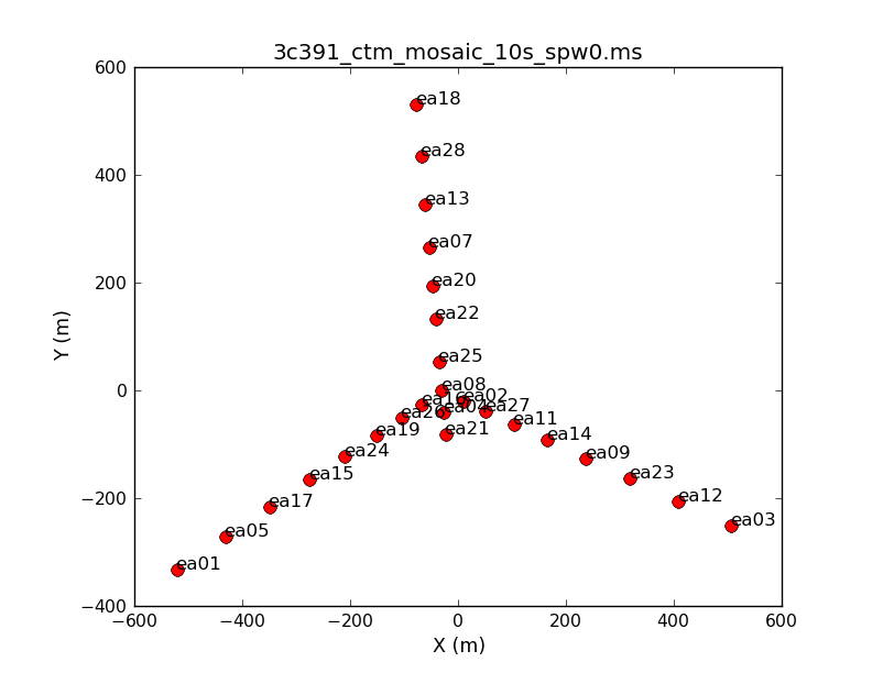
Both to get a sense of the array, as well as identify an antenna for later use in calibration, use the task plotants. In general, for calibration purposes, one would like to select an antenna that is close to the center of the array (and that is not listed in the operator's log as having had problems!).
plotants(vis='3c391_ctm_mosaic_10s.ms',figfile='3c391_ctm_mosaic_antenna_layout.png')
Examining and Editing the Data
It is always a good idea, particularly with a new system like the EVLA, to examine the data. Moreover, from the observer's log, we already know that one antenna will need to be flagged because it does not have a C-band receiver. Start by flagging data known to be bad, then examine the data.
In its current operation, it is common to insert a dummy scan as the first scan. (From the listobs output above, one may have noticed that the first scan is only 10 seconds long.) This first scan can safely be deleted.
flagdata(vis=msname,flagbackup=T,mode='manualflag',selectdata=T,scan='1')
- flagbackup=T : A comment is warranted on the setting of flagbackup (here set to T or True). If set to True, flagdata will save a copy of the existing set of flags before entering any new flags. The setting of flagbackup is therefore a matter of some taste. One could choose not to save any flags or only save "major" flags, or one could save every flag. (One of the authors of this document was glad that flagbackup was set to True as he recently ran flagdata with a typo in one of the entries.)
- mode='manualflag' : Specific data are going to be selected to be edited.
- selectdata=T : In order to select the specific data to be flagged, selectdata has to be set to True. Once selectdata is set to True, then the various data selection options become visible (use inp flagdata to see the possible options). In this case, scan='1' is chosen to select only the first scan. Note that scan expects an entry in the form of a string. (scan=1 would generate an error.)
If satisfied with the inputs, run this task. The initial display in the logger will include
##########################################
##### Begin Task: flagdata           #####
flagdata::::casa
attached MS [...]
Saving current flags to manualflag_2 before applying new flags
Creating new backup flag file called manualflag_2
which indicates that, among other things, the flags that existed in the data set prior to this run will be saved to another file called manualflag_2. Should one ever desire to revert to the data prior to this run, the task flagmanager could be used.
From the observer's log, we know that antenna 13 does not have a C band receiver, so it should be flagged as well. The parameters are similar as before.
flagdata(vis=msname,flagbackup=T,mode='manualflag',selectdata=T,antenna='ea13')
- antenna='ea13' : Once again, this parameter requires a string output. Also note that antenna='ea13' and 'antenna='13' are not the same antenna. (Check the output from listobs above.)
Finally, it is common for the array to require a small amount of time to "settle down" at the start of a scan. Consequently, it has become standard practice to edit out the initial samples from the start of each scan.
flagdata(vis='3c391_ctm_mosaic_10s.ms',mode='quack',quackinterval=10.0,quackmode='beg')
- mode='quack' : Quack is another mode in which the same edit will be applied to all scans for all baselines.
- quackmode='beg' : In this case, data from the start of each scan will be flagged. Other options include flagging data at the end of the scan.
- quackinterval=10 : In this data set, the sampling time is 10 seconds, so this choice flags the first sample from all scans on all baselines.
Having now done some basic editing of the data, based in part on a priori information, it is time to look at the data to determine if there are any other obvious problems. One task to examine the data themselves is plotms.
plotms(vis='3c391_ctm_mosaic_10s.ms',xaxis='',yaxis='',selectdata=True,averagedata=False,transform=False,extendflag=False,plotfile='')
- xaxis=, yaxis= : One can choose the axes of the plot, i.e., the way of visualizing the data.
- selectdata=T : One can choose to plot only subsets of the data.
- averagedata=F : It is possible to average the data in time, frequency, etc.
- transform=F : It is possible to change the velocity reference frame of the data.
- extendflag=F : It is possible to "extend" a flag, i.e., flag data surrounding bad data. For example, one might want to flag spectral channels surrounding a bad spectral channel or one might want to flag cross-polarization data if one flags the parallel polarization data.
- plotfile= : It is possible to produce a hard copy (e.g., for a paper, report, or Web site) by specifying a file.
In this case, most of the values have been left to defaults as it is also possible to select them from within the plotms GUI. Review the inputs, then run the task.
plotms should produce a GUI, with the default view being to show the visibility amplitude as a function of time.
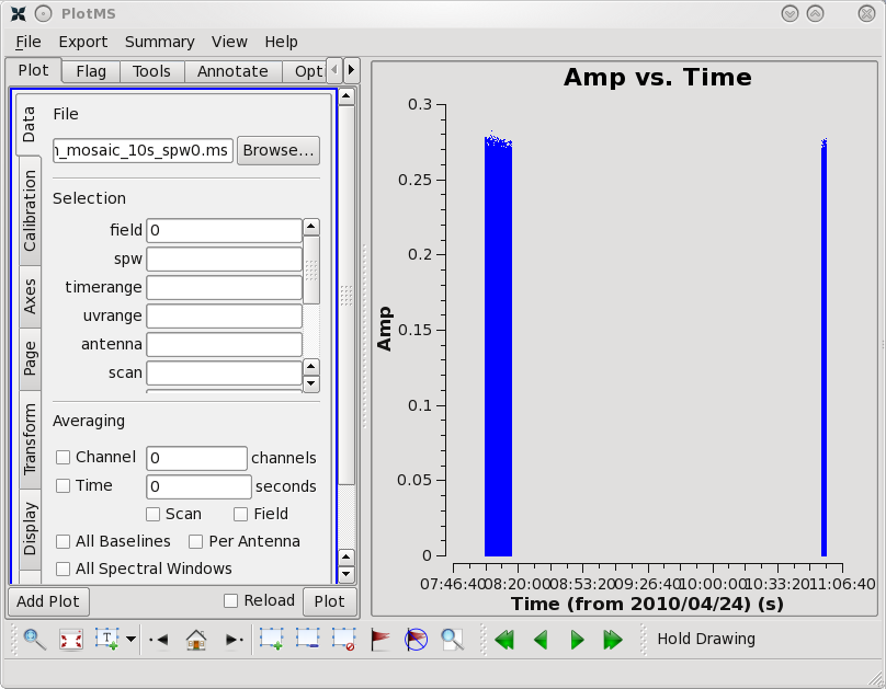
plotms allows one to select and view the data in many ways. Across the top of the right panel are a set of tabs labeled 'Plots', 'Flagging', 'Tools', 'Annotator', and 'Options'. If one selects the 'Flagging' tab, the option is to 'Extend flags'. Thus, even though plotms was started with extendflag=F, if one decides that it does make sense to extend the flags, one can still do so here.
In the default view, the 'Plots' tab is visible, and there are a number of tabs running down the side of the right hand panel, including 'Data', 'Axes', 'Trans', 'Cache', 'Display', 'Canvas', and 'Export'. Once again, one can make changes on the fly. Thus, supposing that one wants to save a hard copy, even if plotms was started with plotfile=, one can select 'Export' and enter a file name in which to save a copy of a plot.
One should spend several minutes displaying the data in various formats. For instance, one could select the 'Data' tab and specify field 0 (source J1331+3030, a.k.a. 3C 286) to display data associated with the amplitude calibrator, then select the 'Axes' tab and change the x axis to be UVDist, and plot the data. The result should be that of the first thumbnail image shown below. The amplitude distribution is relatively constant as a function of u-v distance or baseline length (i.e., sqrt[u*u + v*v]). From the various lectures, one should recognize that a relatively constant visibility amplitude as a function of baseline length means that the source is very nearly a point source. (The Fourier transform of a constant is a delta function, a.k.a. a point source.)
By contrast, if one selects field 3 (one of the 3C 391 fields) in the 'Data' tab and plots these data, one sees a visibility function that falls rapidly with increasing baseline length. Such a visibility function indicates a highly resolved source. By noting the baseline length at which the visibility function falls to some fiducial value (e.g., 1/2 of its peak value), one can obtain a rough estimate of the angular scale of the source. (From the lectures, angular scale [in radians] ~ 1/baseline [in wavelengths].)
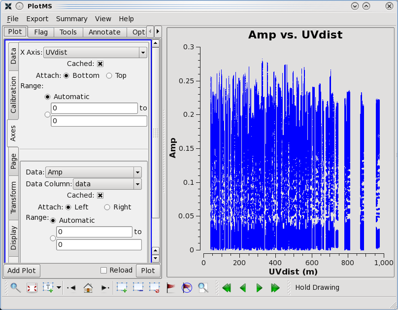
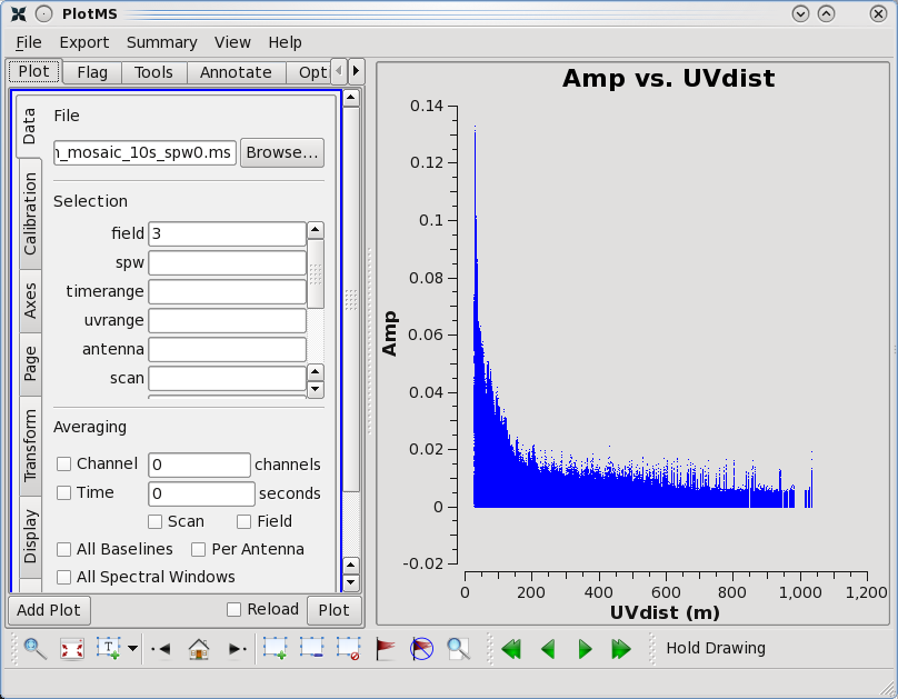
As a general data reduction strategy, one wants to focus at this stage on the calibrators. The data reduction strategy is to determine various corrections from the calibrators, then apply these correction factors to the science data. The 3C 286 data look relatively clean. There are no wildly egregious data (e.g., amplitudes that are 100,000x larger than the rest of the data). One may notice that there are antenna-to-antenna variations (under the 'Display' tab, select 'Colorize by Antenna1'). These antenna-to-antenna variations are acceptable, that's what calibration will help determine.
Calibrating the data
setjy(vis='3c391_ctm_mosaic_10s.ms',field='J1331+3030',spw='0',
    modimage = '/home/casa/data/nrao/VLA/CalModels/3C286_C.im',standard = 'Perley-Taylor 99',
    fluxdensity = -1)

setjy(vis='3c391_ctm_mosaic_10s.ms',field='J1331+3030',spw='1',
    modimage = '/home/casa/data/nrao/VLA/CalModels/3C286_X.im',standard = 'Perley-Taylor 99',
    fluxdensity = -1)
Bandpass calibration
gaincal(vis='3c391_ctm_mosaic_10s.ms',caltable='3c391_ctm_mosaic.gcal0',field='J1331+3030',
    refant='ea21',spw='0~1:27~36',calmode='p')
bandpass(vis='3c391_ctm_mosaic_10s.ms',gaintable='3c391_ctm_mosaic.gcal0',caltable='3c391_ctm_mosaic.bcal0',
    field='J1331+3030',spw='0,1',refant='ea21',solnorm=True,combine='scan',solint='inf',bandtype='B')
Gain calibration
gaincal(vis='3c391_ctm_mosaic_10s.ms',caltable='3c391_ctm_mosaic.gcal1',field='J1331+3030',spw='0,1:5~58'
    refant='ea21',gaintype='G',gaintable='3c391_ctm_mosaic.bcal0',calmode='ap',solint='inf')
gaincal(vis='3c391_ctm_mosaic_10s.ms',caltable='3c391_ctm_mosaic.gcal1',field='J1822-0938,J0319+4130',
    spw='0,1:5~58',refant='ea21',gaintype='G',gaintable='3c391_ctm_mosaic.bcal0',calmode='ap',
    solint='inf',append=True)
Polarization calibration
Now we need to do the polarization calibration. This should be done prior to running fluxscale, since it has to run using the un-rescaled gains in the model data column of the measurement set. Polarization calibration is done in two steps. First, we solve for the instrumental polarization (the frequency-dependent leakage terms, or 'D-terms'), using either an unpolarized source or a source which has sufficiently good parallactic angle coverage. Second, we solve for the polarization position angle using a source with a known polarization position angle (3C 286 is recommended here).
Our initial run of setjy only set the total intensity of our flux calibrator source, 3C 286. This source is known to have a fractional polarization of 11.2% at C-band, and a polarization position angle of 66 degrees.
i0=7.74664
p0=0.112*i0
q0=p0*cos(66*pi/180)
u0=p0*sin(66*pi/180)

i1=5.65053
p1=0.112*i1
q1=p1*cos(66*pi/180)
u1=p1*sin(66*pi/180)

setjy(vis='3c391_ctm_mosaic_10s.ms',field='J1331+3030',modimage='',spw='0',fluxdensity=[i0,q0,u0,0])
setjy(vis='3c391_ctm_mosaic_10s.ms',field='J1331+3030',modimage='',spw='1',fluxdensity=[i1,q1,u1,0])
Solving for the leakage terms
polcal(vis='3c391_ctm_mosaic_10s.ms',caltable='3c391_ctm_mosaic.pcal0',field='J0319+4130',
    spw='0,1',refant='ea21',poltype='Df',gaintable=['3c391_ctm_mosaic.gcal1', '3c391_ctm_mosaic.bcal0'])
Solving for the R-L polarization angle
polcal(vis='3c391_ctm_mosaic_10s.ms',caltable='3c391_ctm_mosaic.xcal0',poltype='Xf',
    gaintable=['3c391_ctm_mosaic.gcal1', '3c391_ctm_mosaic.bcal0', '3c391_ctm_mosaic.pcal0']),
    field='J1331+3030',refant='ea21',spw='0,1')
Applying the calibration
fluxscale(vis='3c391_ctm_mosaic_10s.ms',caltable='3c391_ctm_mosaic.gcal1',fluxtable='3c391_ctm_mosaic.fluxscale1',
    reference='J1331+3030',transfer='J1822-0938,J0319+4130',append=True)
applycal(vis='3c391_ctm_mosaic_10s.ms',
    gaintable=['3c391_ctm_mosaic.fluxscale1','3c391_ctm_mosaic.bcal0','3c391_ctm_mosaic.pcal0','3c391_ctm_mosaic.xcal0'],
    parang=True,field='J1331+3030',gainfield=['J1331+3030','','',''],interp=['nearest','','',''])

applycal(vis='3c391_ctm_mosaic_10s.ms',
    gaintable=['3c391_ctm_mosaic.fluxscale1','3c391_ctm_mosaic.bcal0','3c391_ctm_mosaic.pcal0','3c391_ctm_mosaic.xcal0'],
    parang=True,field='J0319+4130',gainfield=['J0319+4130','','',''],interp=['nearest','','',''])

applycal(vis='3c391_ctm_mosaic_10s.ms',
    gaintable=['3c391_ctm_mosaic.fluxscale1','3c391_ctm_mosaic.bcal0','3c391_ctm_mosaic.pcal0','3c391_ctm_mosaic.xcal0'],
    parang=True,field='J1822-0938',gainfield=['J1822-0938','','',''],interp=['nearest','','',''])
Next, we apply the calibration to the target fields in the mosaic, linearly interpolating the gain solutions from the secondary calibrator, J1822-0938. We can select all 7 fields at once (setting field='2~8').
applycal(vis='3c391_ctm_mosaic_10s.ms',
    gaintable=['3c391_ctm_mosaic.fluxscale1','3c391_ctm_mosaic.bcal0','3c391_ctm_mosaic.pcal0','3c391_ctm_mosaic.xcal0'],
    parang=True,field='2~8',gainfield=['J1822-0938','','',''],interp=['linear','','',''])
Once the calibration has been applied to the target data, we can split off the source, creating a new, calibrated measurement set containing all the target fields. In this case, we also split up the data by spectral window, so we can image the two different frequencies separately.
split(vis='3c391_mosaic_10s.ms',outputvis='3c391_ctm_mosaic_spw0.ms',datacolumn='corrected',field='2~8',spw='0')
split(vis='3c391_mosaic_10s.ms',outputvis='3c391_ctm_mosaic_spw1.ms',datacolumn='corrected',field='2~8',spw='1')
Imaging and self-calibration
Now that we have split off your target data into a separate measurement set with all the calibration applied, it's time to make an image. CASA has a single task, clean which both Fourier transforms the data and deconvolves the resulting image.
A command line call to image and deconvolve the dataset would be:
clean(vis='3c391_ctm_mosaic_spw0.ms',imagename='3c391_ctm_spw0_IQUV',cell=['2.0arcsec','2.0arcsec'],imsize=[576,576],
    mode='mfs',niter=10000,threshold='1.0mJy',stokes='IQUV',psfmode='clarkstokes',
    weighting='briggs',imagermode='mosaic',multiscale=[1,3,10,30,100],mask=[162,177,377,397])
To image the dataset in all four polarizations (total intensity I, linear polarizations Q and U, and circular polarization V), we set stokes='IQUV', which makes separate images in each polarization. We also set psfmode='clarkstokes, which uses the clark clean algorithm to deconvolve each Stokes plane separately. This makes the polarization image more independent of the total intensity.
Since our fractional bandwidth is non-zero (128 MHz at a central frequency of 4.6 GHz), there is a slight improvement in uv-coverage if we do not average all channels together. Our dataset consists of multiple spectral channels, whose data we wish to combine into a single image, gridding each channel separately. We therefore set mode='mfs'.
We need to select the appropriate pixel size to use. Using plotms to look at the newly-calibrated, target-only data set:
plotms(vis='3c391_ctm_mosaic_spw0.ms')
we select the axes tab on the left hand side, and select UVDist_L as the x-axis. This gives the plot shown below
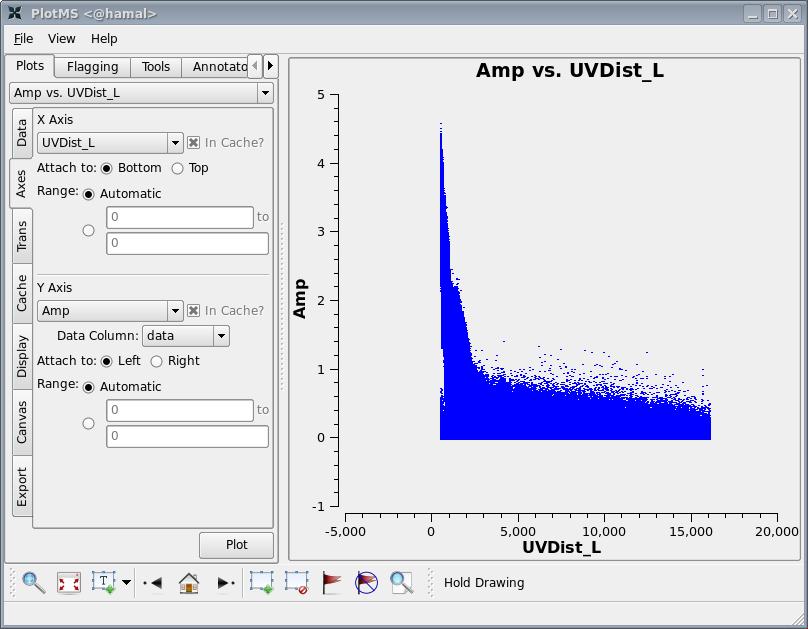
The maximum baseline shown corresponds to about 16,000 wavelengths, i.e. an angular scale of 12 arcseconds ([math]\displaystyle{ \lambda/D=1/16000 }[/math]). Since we wish to have a number of pixels across a resolution element, we then select a pixel size of 2 arcseconds in both co-ordinates by setting cell=['2.0arcsec','2.0arcsec']. The supernova remnant is known to have a diameter of order 9 arcmin, which corresponds to about 270 pixels. To prevent image artifacts arising from aliasing, we wish to keep the emission region to roughly the inner quarter of the image. The Fourier transform is most efficient if the number of pixels on a side is a composite number divisible by 2 and 3 and/or 5. We choose 576, which is [math]\displaystyle{ 2^6\times3^2 }[/math], and is close to [math]\displaystyle{ 2\times270 }[/math]. We therefore set imsize=[576,576].
Since 3C 391 has diffuse, extended emission which is being resolved out by the interferometer owing to a lack of short spacings, a naturally-weighted image would show large-scale patchiness in the noise. In order to suppress this effect, we select Briggs weighting (intermediate between natural and uniform weighting), with a default robust factor of 0 (setting weighting='briggs').
Our data consists of a 7-pointing mosaic, since the supernova remnant fills almost the full primary beam at 4.6 GHz. We therefore wish to perform a joint deconvolution on all 7 fields, which we do simply by setting imagermode='mosaic', and using the default mosaic parameters.
Because the supernova remnant contains both diffuse, extended structure on large spatial scales, and also finer filamentary structure on smaller scales, we use the multiscale clean algorithm, which removes clean components which are circular Gaussians as well as delta functions. We set a logarithmically-spaced range of spatial scales to use for the widths of the Gaussian components, which we specify in pixels. To do this, we set multiscale=[1,3,10,30,100].
To prevent the clean algorithm finding spurious components on noise peaks, especially at the larger scales in the multiscale clean, we set a region within which the task will search for clean components, using mask=[162,177,377,397], which encompasses the observed emission (we can get a rough idea of where the bulk of the emission lies by running clean once with no deconvolution, i.e. niter=0, to make a dirty image, which we can then inspect with the viewer to locate the emission regions). To prevent overcleaning, we wish to stop the deconvolution when we have reached a residual flux level of 1 mJy (setting threshold='1.0mJy'), or when we have generated 10000 clean components (setting niter=10000).
clean will make several output files, all named with the prefix given as imagename. These include:
- .image - the final restored image, with the clean components convolved with a restoring beam and added to the remaining residuals at the end of the imaging process
- .flux - the effective response of the telescope (the primary beam)
- .flux.pbcoverage - the effective response of the full mosaic image
- .mask - the areas where you have permitted imager to find clean components
- .model - the sum of all the clean components, which has been stored as the model_data column in the measurement set
- .psf - the dirty beam, which is being deconvolved from the true sky brightness during the clean process
- .residual - what is left at the end of the deconvolution process; this is useful to diagnose whether or not to clean more deeply
After the imaging and deconvolution process has finished, you can use the viewer to look at your image.
viewer('3c391_ctm_spw0_IQUV.image')
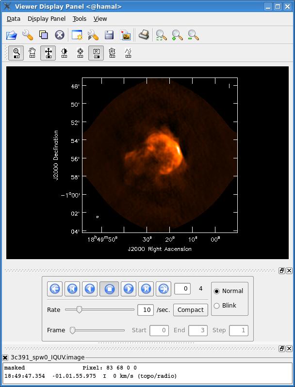
This will bring up a viewer window containing the image, which should look similar to that shown below. The tape deck buttons that you see under the image can be used to step through the different Stokes parameters (I,Q,U,V). You can adjust the color scale and zoom in to a selected region by assigning mouse buttons to the icons immediately above the image (hover over the icons to get a description of what they do).
Note that the image is cut off in a circular fashion at the edges, corresponding to the default minimum primary beam response within clean of 0.2.
