Protoplanetary Disk Simulation - VLA-CASA5.3.0
VLA version: under construction!!!
CASA <253>: inp
> inp()
- simobserve :: visibility simulation task
project = 'psimvla' # root prefix for output file names skymodel = 'ppdisk43_GHz_50pc.fits' # model image to observe
    inbright       =                 #  scale surface brightness of brightest pixel e.g. "1.2Jy/pixel"
    indirection    =                 #  set new direction e.g. "J2000 19h00m00 -40d00m00"
    incell         =                 #  set new cell/pixel size e.g. "0.1arcsec"
    incenter       =                 #  set new frequency of center channel e.g. "89GHz" (required even for 2D model)
    inwidth        =     '8GHz'        #  set new channel width e.g. "10MHz" (required even for 2D model)
complist = # componentlist to observe setpointings = True
    integration    =       '3s'        #  integration (sampling) time
    direction      = 'J2000 18h00m00.031s -22d59m59.6s' #  "J2000 19h00m00 -40d00m00" or "" to center on model
    mapsize        = '0.76arcsec'      #  angular size of map or "" to cover model
    maptype        =   'square'        #  hexagonal, square (raster), ALMA, etc
    pointingspacing =                #  spacing in between pointings or "0.25PB" or "" for ALMA default INT=lambda/D/sqrt(3), SD=lambda/D/3
obsmode = 'int' # observation mode to simulate [int(interferometer)|sd(singledish)|""(none)]
    antennalist    = 'vla.a.cfg'       #  interferometer antenna position file
    refdate        = '2014/05/21'      #  date of observation - not critical unless concatting simulations
    hourangle      =  'transit'        #  hour angle of observation center e.g. "-3:00:00", "5h", "-4.5" (a number without units will be interpreted as
                                       #   hours), or "transit"
    totaltime      =   '12000s'        #  total time of observation or number of repetitions
    caldirection   =                 #  pt source calibrator [experimental]
    calflux        =      '1Jy'
outframe = 'LSRK' # spectral frame of MS to create thermalnoise = 'tsys-atm' # add thermal noise: [tsys-atm|tsys-manual|""]
    user_pwv       =          4        #  Precipitable Water Vapor in mm
    t_ground       =      270.0        #  ambient temperature
    seed           =      11111        #  random number seed
leakage = 0.0 # cross polarization (interferometer only) graphics = 'both' # display graphics at each stage to [screen|file|both|none] verbose = False overwrite = True # overwrite files starting with $project
=
CASA <255>: inp
> inp()
- simanalyze :: image and analyze measurement sets created with simobserve
project = 'psimvla' # root prefix for output file names image = True # (re)image $project.*.ms to $project.image
    vis            = 'psimvla.vla.a.noisy.ms' #  Measurement Set(s) to image
    modelimage     = 'ppdisk43_GHz_50pc.fits' #  lower resolution prior image to use in clean e.g. existing total power image
    imsize         = [192, 192]        #  output image size in pixels (x,y) or 0 to match model
    imdirection    =                 #  set output image direction, (otherwise center on the model)
    cell           =                 #  cell size with units e.g. "10arcsec" or "" to equal model
    interactive    =      False        #  interactive clean?  (make sure to set niter>0 also)
    niter          =          1        #  maximum number of iterations (0 for dirty image)
    threshold      =   '1e-7Jy'        #  flux level (+units) to stop cleaning
    weighting      =  'uniform'        #  weighting to apply to visibilities.  briggs will use robust=0.5
    mask           =         []        #  Cleanbox(es), mask image(s), region(s), or a level
    outertaper     =         []        #  uv-taper on outer baselines in uv-plane
    pbcor          =       True        #  correct the output of synthesis images for primary beam response?
    stokes         =        'I'        #  Stokes params to image
    featherimage   =                 #  image (e.g. total power) to feather with new image
analyze = True # (only first 6 selected outputs will be displayed)
    showuv         =      False        #  display uv coverage
    showpsf        =       True        #  display synthesized (dirty) beam (ignored in single dish simulation)
    showmodel      =       True        #  display sky model at original resolution
    showconvolved  =       True        #  display sky model convolved with output clean beam
    showclean      =       True        #  display the synthesized image
    showresidual   =       True        #  display the clean residual image (ignored in single dish simulation)
    showdifference =       True        #  display difference between output cleaned image and input model sky image convolved with output clean beam
    showfidelity   =       True        #  display fidelity (see help)
graphics = 'both' # display graphics at each stage to [screen|file|both|none] verbose = True overwrite = True # overwrite files starting with $project dryrun = False # only print information [experimental; only for interfermetric data] logfile =
Protoplanetary Disk Simulation - VLA
- This is an advanced simulation tutorial. New users are recommended to begin with reading the CASA Docs documentation pages on "Simulations".
- This guide is applicable to CASA version 5.1.
- To create a script of the Python code on this page see Extracting scripts from these tutorials.
Data
For this CASA Guide we will use a protoplanetary disk model from S. Wolf. Get the data here. Note that this is a modified image from the ALMA Simulation Inputs, where we changed the center frequency 35GHz and the bandwidth to 128MHz. '
Script with Explanation
Set simobserve as the current task and reset all parameters.
# In CASA
default("simobserve")
Let's call our project "psimvla". This defines the root prefix for any output files from simobserve.
project = "psimvla"
Review the image coordinate system using task imhead.
# This reports image header parameters in the Log Messages window
imhead("ppdisk43_GHz_50pc.fits")
This confirms that the data are set at 43GHz center frequency with a bandwidth of 128MHz. Note that the reference coordinate of the image is at pixel (0,0), i.e. in a corner of the image, not the center. In [[1]] a method is provided on how to derive the image centers through the toolkit. Using that method, or inspecting the image with the viewer shows that the image center is at RA=18h00m00.031s, DEC=-22d59m59.6s.
We'll set skymodel to the FITS file downloaded, above, and leave all skymodel subparameters at their default values. simobserve will create CASA image psimvla.skymodel.
skymodel = "ppdisk43_GHz_50pc.fits"
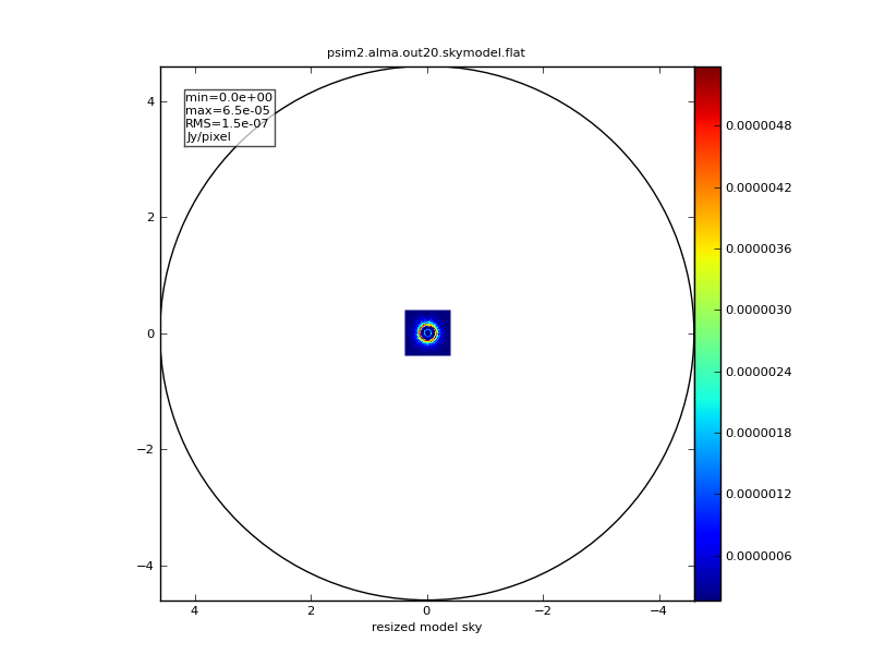
We will specify the sky position for the center of the observation and set the map size to the size of the model image. The image is very small compared to the VLA primary beam at 35GHz () Since the model image is 2/3 arcseconds across, we should only need one pointing. In this case, pointingspacing and maptype can be left at their default values.
setpointings       =  True
direction          =  "J2000 18h00m00.031s -22d59m59.6s"
mapsize            =  "0.76arcsec"
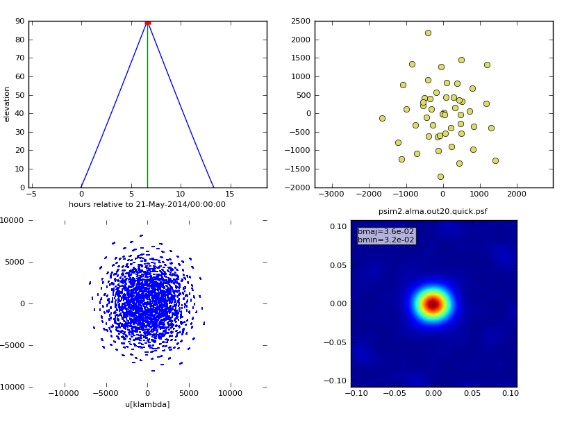
We do want to simulate an interferometric observation, so we set obsmode accordingly. We'll set totaltime to a 20-minute snapshot observation.
obsmode            =  "int"
totaltime          =  "1200s"
We want to use the appropriate antenna configuration for the desired angular resolution. Configuration 20, alma.out20.cfg, is the largest "compact" configuration. A list of configuration files available in CASA 4.1 is available here.
antennalist = "vla.a.cfg"
We do not want to simulate observations with thermal noise in this example, so we set:
thermalnoise = ''
Now run simobserve.
simobserve()
Now that we've simulated the visibility measurements, we want to generate an image from the simulated data. simanalyze makes this easy. We begin by setting project to the same prefix used in simobserve and setting image to True.
default ("simanalyze")
project = "psimvla"
image = True
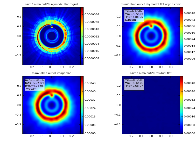
We set modelimage to use the input FITS image when cleaning the simulated visibilities. We set the image size to 192 pixels square.
modelimage = "ppdisk43_GHz_50pc.fits"
vis = project + ".vla.a.ms"
imsize = [192, 192]
Specify the number of iterations for cleaning, with proper threshold and weighting.
niter = 10000
threshold = "1e-7Jy"
weighting = "natural"
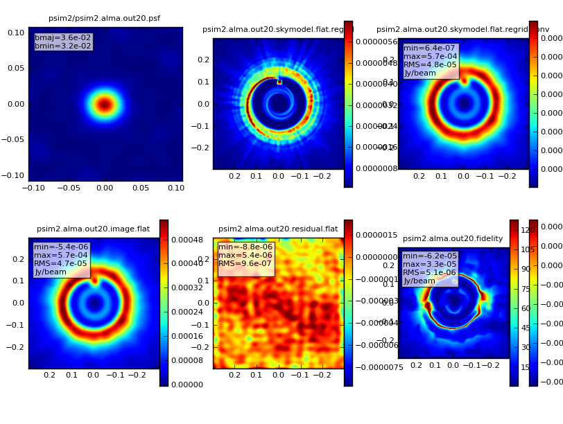
We'd like to calculate a difference and fidelity image, but we don't need to see the uv coverage.
analyze = True
showuv = False
showresidual = True
showconvolved = True
Plot both to the screen and PNG files with lots of messages.
graphics = "both"
verbose = True
overwrite = True
Run simanalyze.
simanalyze()
Simulation Output
Input:
|
simobserve:
|
simanalyze image:
|
simanalyze output:
|