Image Line CASA 6.1.1
This guide continues from Image_Continuum and Self_Calibration_Template (optional). Imaging parameters and calibration tables (if applicable) should already be set prior to continuing.
Continuum Subtraction for Line Emission
If you have observations that include both line and strong continuum emission (>3 sigma above the noise), you need to subtract the continuum from the line data. You should not subtract the continuum from the line data if the line of interest is an absorption line. You will need to insert any continuum spws that weren’t included in flagchannels. For example, if your continuum spws are '0,1,2' and flagchannels='1:260~500', au.invertChannelRanges will return '1:0~259,1:501~3839'. The fitspw parameter should be '0,1:0~259,1:501~3839,2'.
Continuum subtraction is done for each field in turn; however, if the fields have different line free channels, then the continuum subtraction will need to be done separately for each field.
# in CASA
fitspw = '2:1201~2199,3:1201~2199' # line free channels. Use au.invertChannelRanges
linespw = '2,3' # line spectral windows. You can subtract the continuum from multiple spectral line windows at once.

finalvis='calibrated_final.ms'

uvcontsub(vis=finalvis,
          spw=linespw, # spw to do continuum subtraction on
          fitspw=fitspw, # regions with lines. can be set equal to flagchannels
          excludechans=False,
          combine='spw',
          solint='int',
          fitorder=1,
          want_cont=False) # This value should not be changed.
Apply continuum self-calibration to line data (optional)
This section depends on solutions derived with Self_Calibration_Template. Skip to Image_Line#Image_line_emission_.28repeat_as_necessary.29 Image Line Emissions (repeat as necessary) if you do not wish to apply self-calibration solutions to the line data.
If you find self-calibration does help with lowering the rms in your continuum images, it is a good idea to apply the continuum self-calibration to the line data. Depending on if you performed continuum subtraction, select the definition of linevis accordingly. Once this has been done, it is recommended that you save the flags before you apply the self-calibration solution to the individual line spectral windows, in case you do not like results or they do not improve the image. If self-calibration of the continuum does improve the quality of those data, apply the derived gaintable to the spectral line channels using the applycal task. This will improve the image quality of the stronger spectral line channels, but will not help (or harm) the weaker line channels. Then save the results of self-cal in a new ms and reset the image name. You also need to reset the corrected data column in the ms to the original calibration. The clearcal(linevis) task can also be used to return your ms to its original pre-self-cal state, if you are dissatisfied with the self-calibration results.
# in CASA
# Uncomment one of the following:
# linevis = finalvis+'.contsub' # if continuum subtracted
# linevis = finalvis  #  if not continuum subtracted
# save original flags in case you don't like the self-cal
flagmanager(vis=linevis,mode='save',versionname='before_selfcal',merge='replace')

spwmap_line = [0] # Mapping self-calibration solution to the individual line spectral windows.
applycal(vis=linevis,
         spwmap=[spwmap_line, spwmap_line], # entering the appropriate spwmap_line value for each spw in the input dataset
         field=field,
         gaintable=['pcal3','apcal'],
         gainfield='',
         calwt=False,
         flagbackup=False)

# Save results of self-cal in a new ms and reset the image name.
split(vis=linevis,
      outputvis=linevis+'.selfcal',
      datacolumn='corrected')
Image line emission (repeat as necessary)
You should now have a measurement set that is ready to image in velocity mode to create line cubes. Depending on the observation, the measurement set may have a variety of names. Make sure to select the correct option below.
# in CASA
finalvis = 'calibrated_final.ms'

# uncomment if you have neither continuum subtracted nor self-calibrated your data
# linevis = finalvis
# uncomment if you have continuum subtracted your data
# linevis = finalvis + ‘.contsub’
# uncomment if you have both continuum subtracted and self-calibrated your data
# linevis = finalvis + '.contsub.selfcal'
# uncomment if you have only self-calibrated your data
# linevis = finalvis + '.selfcal'
Now the linevis variable will be used for the rest of the cleaning. Spectral windows and field numbers may have been re-numbered. Check for these changes.
# in CASA
vishead(linevis)
Set the necessary parameters for clean. The name of the image will be formated as sourcename_linetransition.
# in CASA
sourcename ='n253' # name of source
linename = 'CO10' # name of transition
lineimagename = sourcename+'_'+linename # name of line image
The restfreq is typically set at the rest frequency of the line of interest. We do not recommend imaging multiple spectral windows tuned to different frequencies. If the source is significantly redshifted (z>0.2), use the observed sky frequency (nu_rest/1+z) instead. If cvel or mstransform was used to regrid spectral windows, make sure to use the same values below.
# in CASA
restfreq='115.27120GHz’
Select the spw you would like to image. If you have multiple executions, you will need to select the spws at the same rest frequency.
# in CASA
spw = ‘0’ # update to the spw you would like to image
The start, width, and nchan parameters will determine the size of the cube you create. Setting the values at their defaults will image the entire spectral window at the native resolution.
# in CASA
start = ‘’
width = ‘’
nchan = -1
You can also image a subset of the cube. For example, you may wish to image the inner 100 channels at a spectral resolution of 2 km/s.
# in CASA
start='-100km/s'
width='2km/s'
nchan = 100
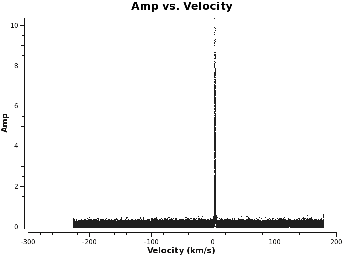
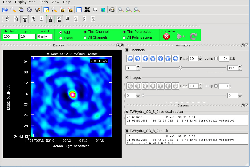
You can use plotms to find the line if it is apparent in the visibilities. <figure id="TWHydra_CO3_2_plotms.png">
</figure> <figure id="CO_initial_image.png">
</figure>
# in CASA
plotms(vis=linevis,xaxis=’velocity’,yaxis=’amp’,avgtime=’1e8’,avgscan=True,avgantenna=True,spw=spw,coloraxis=’spw’,transform=True,freqframe=outframe.upper(),restfreq=restfreq)
The following commands can be run to re-start the cleaning process from scratch if you have already created a cube.
# in CASA
clearcal(vis=linevis)
delmod(vis=linevis)
for ext in ['.flux','.image','.mask','.model','.pbcor','.psf','.residual','.flux.pbcoverage','.pb','.wtsum']:
    rmtables(lineimagename + ext)
The First Look at Spectral Line Imaging guide can be used for first time imagers. Check out the tips and tricks for imaging in the continuum imaging section of this guide.
# in CASA
clean(vis=linevis,
      imagename=lineimagename,
      field=field,
      spw=spw,
#      phasecenter=phasecenter, # uncomment if mosaic.
      mode='velocity',
      start=start,
      width=width,
      nchan=nchan,
      outframe=outframe,
      veltype=veltype,
      restfreq=restfreq,
      niter=niter,
      threshold=threshold,
      interactive=True,
      cell=cell,
      imsize=imsize,
      weighting=weighting,
      robust=robust,
      imagermode=imagermode)
You can use this template to image all targeted lines in your observation.
Apply a primary beam correction
<figure id="TW_Hya_Calibrated_final_cont.image.png">
</figure> <figure id="TW_Hya_Calibrated_final.pbcor.png">
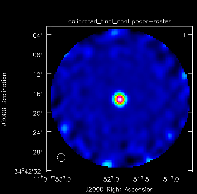
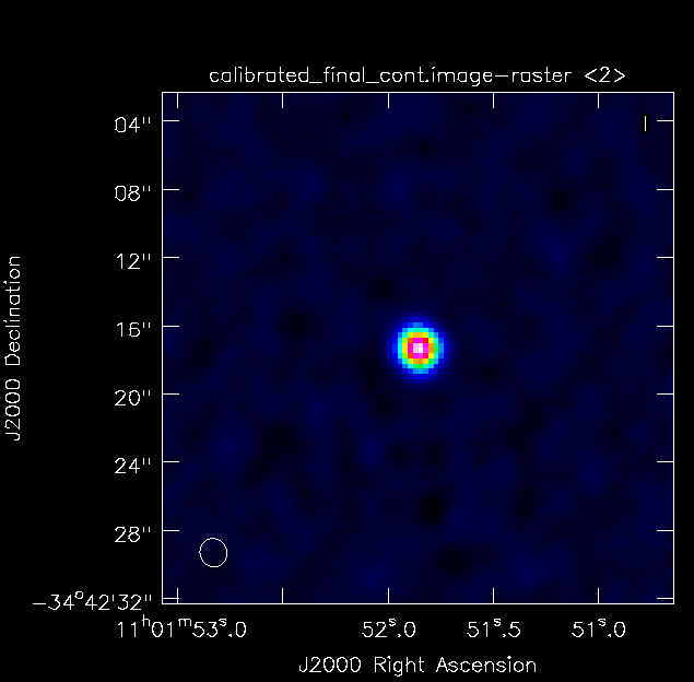
</figure> Once all imaging is finished, diagnostic images will be made. The first of these is a primary beam correction image of the data. Each telescope's primary beam is, for the most part, approximately a Gaussian with small side lobes that can be approximated to zero. Because of this, the center of the beam has much more sensitivity than the edges. To correct for this, flux is added to the edges of the image in order for all pixels across the beam to have the same relative brightness based on the beam pattern.
impbcor is used to produce the primary beam corrected images . You will need the *.flux and *.pbcor files.
# in CASA
import glob

myimages = glob.glob("*.image")

rmtables('*.pbcor')
for image in myimages:
	pbimage = image.rsplit('.',1)[0]+'.flux'
	outfile = image.rsplit('.',1)[0]+'.pbcor'
	impbcor(imagename=image, pbimage=pbimage, outfile = outfile)
Export the images
Use exportfits to create fits files of the *.flux and *.pbcor files.
# in CASA
import glob

myimages = glob.glob("*.pbcor")
for image in myimages:
    exportfits(imagename=image, fitsimage=image+'.fits',overwrite=True)

myimages = glob.glob("*.flux")
for image in myimages:
    exportfits(imagename=image, fitsimage=image+'.fits',overwrite=True)
Create Diagnostic PNGs
<figure id="TWHydra_CO_3_2.image.mom8.png">
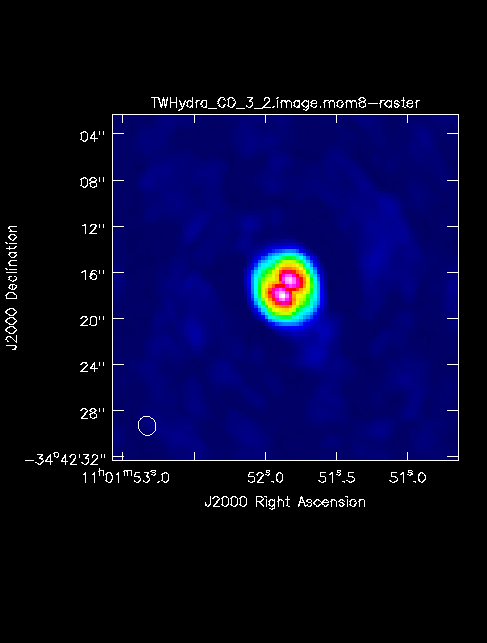
</figure> The First Look at Image Analysis guide gives an introduction to a variety of options to begin image analysis, including using immoments to create moment maps. The commands create png files of the continuum image and moment 8 maps.
# in CASA
os.system("rm -rf *.png")
mycontimages = glob.glob("calibrated*.image")
for cimage in mycontimages:
    max=imstat(cimage)['max'][0]
    min=-0.1*max
    outimage = cimage+'.png'
    os.system('rm -rf '+outimage)
    imview(raster={'file':cimage,'range':[min,max]},out=outimage)


# this will have to be run for each sourcename
sourcename='' # insert source here, if it isn't already set
mylineimages = glob.glob(sourcename+"*.image")
for limage in mylineimages:
    rms=imstat(limage,chans='1')['rms'][0]
    mom8=limage+'.mom8'
    os.system("rm -rf "+mom8)
    immoments(limage,moments=[8],outfile=mom8)
    max=imstat(mom8)['max'][0]
    min=-0.1*max
    os.system("rm "+mom8+".png")
    imview(raster={'file':mom8,'range':[min,max]},out=mom8+'.png')