VLA CASA Bandpass Slope-CASA4.5.2
This CASA Guide is for CASA version 4.5.2
Overview
For the standard VLA flux density calibrators 3C138, 3C147, 3C286, and 3C48, CASA includes a spatial and spectral model that is applied for bandpass calibration. This model removed the source characteristics, resulting in a calibration solution that is a representation of the instrumental and atmospheric corrections. These VLA standard calibrators, however, exhibit a negative spectral index and are relatively weak at high frequencies.
Although the standard VLA flux density calibrators are usually still bright enough for absolute flux density calibration, a good bandpass determination—which is very important for spectral line observations—requires large signal-to-noise ratios derived from either a long integration time or a very strong source (see the Spectral Line Guide for Observing). Observations of non-standard, but strong, bandpass calibrators are therefore common at high frequencies. Unfortunately, such sources are likely variable and no a priori flux density model is available. In particular, these sources exhibit an unknown and maybe variable spectral slope, which, if not accounted for, will create an error in the bandpass calibration. This tutorial describes how to model a spectral slope and how to correct the bandpass solution for this effect.
Data used in this guide are taken in wide 3-bit mode for the protostar G192.16-3.84 in Ka-band with basebands centered at 29 and 36.5 GHz. Each baseband has over 4 GHz of bandwidth comprising thirty-two 128-MHz spectral windows.
If you are new to CASA, or with VLA data reduction in CASA, it is strongly recommended that you start with either the EVLA Continuum Tutorial 3C391 or Getting Started in CASA before proceeding with this tutorial.
Obtaining the Data
As this tutorial concerns bandpass calibration, all sources other than the flux density and bandpass calibrator scans were removed from the MS. All pre-calibration steps including flagging, antenna position offsets, requantizer gains, opacity corrections, and gain-elevation curves were applied. The original data (TVER0004.sb14459364.eb14492359.56295.26287841435) can be obtained through the NRAO archive and has a raw size of 57.04 GB.
The trimmed measurement set can be downloaded directly from http://casa.nrao.edu/Data/EVLA/G192/G192-BP.ms.tar.gz (dataset size: 3.4 GB)
Your first step will be to unzip and untar the file in a terminal (before you start CASA):
tar -xzvf G192-BP.ms.tar.gz
Starting CASA
To start CASA, type:
casa
This will run a script initializing CASA and setting paths appropriately. The script will also create two files called ipython-<unique-stamp>.log (which contains a record of all the text you enter at the CASA prompt) as well as casapy-<unique-stamp>.log (which will contain all the messages that are printed to the CASA logger window). It is recommended that you keep your log files intact—you may need them to remind you of the last step you completed in your data reduction. (It is also a good idea to include your log files when submitting a help desk ticket).
Once CASA has started, a logger window will appear. Note that you can rescale this window or change the font size (under the View menu option) as desired.
Examining the Measurement Set (MS)
We use listobs to summarize our MS:
# In CASA: listobs on the initial data set
listobs('G192-BP.ms', listfile='G192_listobs.txt')
This will write the output to a file called G192_listobs.txt, which we can print to the terminal using various Unix/Linux commands such as cat, less, or more:
# In CASA
cat G192_listobs.txt
================================================================================
MeasurementSet Name: /lustre/aoc/sciops/jott/casa/topicalguide/bandpass/new/G192-BP.ms MS Version 2
================================================================================
Observer: Dr. Debra Shepherd Project: uid://evla/pdb/7303457
Observation: EVLA
Data records: 1769355 Total elapsed time = 4563 seconds
Observed from 03-Jan-2013/06:31:48.0 to 03-Jan-2013/07:47:51.0 (UTC)
ObservationID = 0 ArrayID = 0
Date Timerange (UTC) Scan FldId FieldName nRows SpwIds Average Interval(s) ScanIntent
03-Jan-2013/06:31:48.0 - 06:36:42.0 6 0 3C147 704865 [0,1,2,3,4,5,6,7,8,9,10,11,12,13,14,15,16,17,18,19,20,21,22,23,24,25,26,27,28,29,30,31,32,33,34,35,36,37,38,39,40,41,42,43,44,45,46,47,48,49,50,51,52,53,54,55,56,57,58,59,60,61,62,63] [6, 6, 6, 6, 6, 6, 6, 6, 6, 6, 6, 6, 6, 6, 6, 6, 6, 6, 6, 6, 6, 6, 6, 6, 6, 6, 6, 6, 6, 5.94, 6, 6, 6, 6, 6, 6, 6, 6, 6, 6, 6, 6, 6, 6, 6, 6, 6, 6, 6, 6, 6, 6, 6, 6, 6, 6, 6, 6, 6, 6, 6, 6, 6, 6] [CALIBRATE_FLUX#UNSPECIFIED,OBSERVE_TARGET#UNSPECIFIED]
07:40:27.0 - 07:47:51.0 64 1 3c84-J0319+413 1064490 [0, 1, 2, 3, 4, 5, 6, 7, 8, 9, 10, 11, 12, 13, 14, 15, 16, 17, 18, 19, 20, 21, 22, 23, 24, 25, 26, 27, 28, 29, 30, 31, 32, 33, 34, 35, 36, 37, 38, 39, 40, 41, 42, 43, 44, 45, 46, 47, 48, 49, 50, 51, 52, 53, 54, 55, 56, 57, 58, 59, 60, 61, 62, 63] [6, 6, 6, 6, 6, 6, 6, 6, 6, 6, 6, 6, 6, 6, 6, 6, 6, 6, 6, 6, 6, 6, 6, 6, 6, 6, 6, 6, 6, 6, 6, 6, 6, 6, 6, 6, 6, 6, 6, 6, 6, 6, 6, 6, 6, 6, 6, 6, 6, 6, 6, 6, 6, 6, 6, 6, 6, 6, 6, 6, 6, 6, 6, 6] [CALIBRATE_BANDPASS#UNSPECIFIED,OBSERVE_TARGET#UNSPECIFIED]
(nRows = Total number of rows per scan)
Fields: 2
ID Code Name RA Decl Epoch SrcId nRows
0 E 3C147 05:42:36.137916 +49.51.07.23356 J2000 0 704865
1 F 3c84-J0319+413 03:19:48.160102 +41.30.42.10305 J2000 1 1064490
Spectral Windows: (64 unique spectral windows and 1 unique polarization setups)
SpwID Name #Chans Frame Ch0(MHz) ChanWid(kHz) TotBW(kHz) CtrFreq(MHz) BBC Num Corrs
0 EVLA_KA#A1C1#2 128 TOPO 34476.000 1000.000 128000.0 34539.5000 10 RR LL
1 EVLA_KA#A1C1#3 128 TOPO 34604.000 1000.000 128000.0 34667.5000 10 RR LL
2 EVLA_KA#A1C1#4 128 TOPO 34732.000 1000.000 128000.0 34795.5000 10 RR LL
3 EVLA_KA#A1C1#5 128 TOPO 34860.000 1000.000 128000.0 34923.5000 10 RR LL
4 EVLA_KA#A1C1#6 128 TOPO 34988.000 1000.000 128000.0 35051.5000 10 RR LL
5 EVLA_KA#A1C1#7 128 TOPO 35116.000 1000.000 128000.0 35179.5000 10 RR LL
6 EVLA_KA#A1C1#8 128 TOPO 35244.000 1000.000 128000.0 35307.5000 10 RR LL
7 EVLA_KA#A1C1#9 128 TOPO 35372.000 1000.000 128000.0 35435.5000 10 RR LL
8 EVLA_KA#A1C1#10 128 TOPO 35500.000 1000.000 128000.0 35563.5000 10 RR LL
9 EVLA_KA#A1C1#11 128 TOPO 35628.000 1000.000 128000.0 35691.5000 10 RR LL
10 EVLA_KA#A1C1#12 128 TOPO 35756.000 1000.000 128000.0 35819.5000 10 RR LL
11 EVLA_KA#A1C1#13 128 TOPO 35884.000 1000.000 128000.0 35947.5000 10 RR LL
12 EVLA_KA#A1C1#14 128 TOPO 36012.000 1000.000 128000.0 36075.5000 10 RR LL
13 EVLA_KA#A1C1#15 128 TOPO 36140.000 1000.000 128000.0 36203.5000 10 RR LL
14 EVLA_KA#A1C1#16 128 TOPO 36268.000 1000.000 128000.0 36331.5000 10 RR LL
15 EVLA_KA#A1C1#17 128 TOPO 36396.000 1000.000 128000.0 36459.5000 10 RR LL
16 EVLA_KA#A2C2#18 128 TOPO 36476.000 1000.000 128000.0 36539.5000 11 RR LL
17 EVLA_KA#A2C2#19 128 TOPO 36604.000 1000.000 128000.0 36667.5000 11 RR LL
18 EVLA_KA#A2C2#20 128 TOPO 36732.000 1000.000 128000.0 36795.5000 11 RR LL
19 EVLA_KA#A2C2#21 128 TOPO 36860.000 1000.000 128000.0 36923.5000 11 RR LL
20 EVLA_KA#A2C2#22 128 TOPO 36988.000 1000.000 128000.0 37051.5000 11 RR LL
21 EVLA_KA#A2C2#23 128 TOPO 37116.000 1000.000 128000.0 37179.5000 11 RR LL
22 EVLA_KA#A2C2#24 128 TOPO 37244.000 1000.000 128000.0 37307.5000 11 RR LL
23 EVLA_KA#A2C2#25 128 TOPO 37372.000 1000.000 128000.0 37435.5000 11 RR LL
24 EVLA_KA#A2C2#26 128 TOPO 37500.000 1000.000 128000.0 37563.5000 11 RR LL
25 EVLA_KA#A2C2#27 128 TOPO 37628.000 1000.000 128000.0 37691.5000 11 RR LL
26 EVLA_KA#A2C2#28 128 TOPO 37756.000 1000.000 128000.0 37819.5000 11 RR LL
27 EVLA_KA#A2C2#29 128 TOPO 37884.000 1000.000 128000.0 37947.5000 11 RR LL
28 EVLA_KA#A2C2#30 128 TOPO 38012.000 1000.000 128000.0 38075.5000 11 RR LL
29 EVLA_KA#A2C2#31 128 TOPO 38140.000 1000.000 128000.0 38203.5000 11 RR LL
30 EVLA_KA#A2C2#32 128 TOPO 38268.000 1000.000 128000.0 38331.5000 11 RR LL
31 EVLA_KA#A2C2#33 128 TOPO 38396.000 1000.000 128000.0 38459.5000 11 RR LL
32 EVLA_KA#B1D1#34 128 TOPO 26976.000 1000.000 128000.0 27039.5000 13 RR LL
33 EVLA_KA#B1D1#35 128 TOPO 27104.000 1000.000 128000.0 27167.5000 13 RR LL
34 EVLA_KA#B1D1#36 128 TOPO 27232.000 1000.000 128000.0 27295.5000 13 RR LL
35 EVLA_KA#B1D1#37 128 TOPO 27360.000 1000.000 128000.0 27423.5000 13 RR LL
36 EVLA_KA#B1D1#38 128 TOPO 27488.000 1000.000 128000.0 27551.5000 13 RR LL
37 EVLA_KA#B1D1#39 128 TOPO 27616.000 1000.000 128000.0 27679.5000 13 RR LL
38 EVLA_KA#B1D1#40 128 TOPO 27744.000 1000.000 128000.0 27807.5000 13 RR LL
39 EVLA_KA#B1D1#41 128 TOPO 27872.000 1000.000 128000.0 27935.5000 13 RR LL
40 EVLA_KA#B1D1#42 128 TOPO 28000.000 1000.000 128000.0 28063.5000 13 RR LL
41 EVLA_KA#B1D1#43 128 TOPO 28128.000 1000.000 128000.0 28191.5000 13 RR LL
42 EVLA_KA#B1D1#44 128 TOPO 28256.000 1000.000 128000.0 28319.5000 13 RR LL
43 EVLA_KA#B1D1#45 128 TOPO 28384.000 1000.000 128000.0 28447.5000 13 RR LL
44 EVLA_KA#B1D1#46 128 TOPO 28512.000 1000.000 128000.0 28575.5000 13 RR LL
45 EVLA_KA#B1D1#47 128 TOPO 28640.000 1000.000 128000.0 28703.5000 13 RR LL
46 EVLA_KA#B1D1#48 128 TOPO 28768.000 1000.000 128000.0 28831.5000 13 RR LL
47 EVLA_KA#B1D1#49 128 TOPO 28896.000 1000.000 128000.0 28959.5000 13 RR LL
48 EVLA_KA#B2D2#50 128 TOPO 28976.000 1000.000 128000.0 29039.5000 14 RR LL
49 EVLA_KA#B2D2#51 128 TOPO 29104.000 1000.000 128000.0 29167.5000 14 RR LL
50 EVLA_KA#B2D2#52 128 TOPO 29232.000 1000.000 128000.0 29295.5000 14 RR LL
51 EVLA_KA#B2D2#53 128 TOPO 29360.000 1000.000 128000.0 29423.5000 14 RR LL
52 EVLA_KA#B2D2#54 128 TOPO 29488.000 1000.000 128000.0 29551.5000 14 RR LL
53 EVLA_KA#B2D2#55 128 TOPO 29616.000 1000.000 128000.0 29679.5000 14 RR LL
54 EVLA_KA#B2D2#56 128 TOPO 29744.000 1000.000 128000.0 29807.5000 14 RR LL
55 EVLA_KA#B2D2#57 128 TOPO 29872.000 1000.000 128000.0 29935.5000 14 RR LL
56 EVLA_KA#B2D2#58 128 TOPO 30000.000 1000.000 128000.0 30063.5000 14 RR LL
57 EVLA_KA#B2D2#59 128 TOPO 30128.000 1000.000 128000.0 30191.5000 14 RR LL
58 EVLA_KA#B2D2#60 128 TOPO 30256.000 1000.000 128000.0 30319.5000 14 RR LL
59 EVLA_KA#B2D2#61 128 TOPO 30384.000 1000.000 128000.0 30447.5000 14 RR LL
60 EVLA_KA#B2D2#62 128 TOPO 30512.000 1000.000 128000.0 30575.5000 14 RR LL
61 EVLA_KA#B2D2#63 128 TOPO 30640.000 1000.000 128000.0 30703.5000 14 RR LL
62 EVLA_KA#B2D2#64 128 TOPO 30768.000 1000.000 128000.0 30831.5000 14 RR LL
63 EVLA_KA#B2D2#65 128 TOPO 30896.000 1000.000 128000.0 30959.5000 14 RR LL
Sources: 128
ID Name SpwId RestFreq(MHz) SysVel(km/s)
0 3C147 0 - -
0 3C147 1 - -
0 3C147 2 - -
0 3C147 3 - -
0 3C147 4 - -
0 3C147 5 - -
0 3C147 6 - -
0 3C147 7 - -
0 3C147 8 - -
0 3C147 9 - -
0 3C147 10 - -
0 3C147 11 - -
0 3C147 12 - -
0 3C147 13 - -
0 3C147 14 - -
0 3C147 15 - -
0 3C147 16 - -
0 3C147 17 - -
0 3C147 18 - -
0 3C147 19 - -
0 3C147 20 - -
0 3C147 21 - -
0 3C147 22 - -
0 3C147 23 - -
0 3C147 24 - -
0 3C147 25 - -
0 3C147 26 - -
0 3C147 27 - -
0 3C147 28 - -
0 3C147 29 - -
0 3C147 30 - -
0 3C147 31 - -
0 3C147 32 - -
0 3C147 33 - -
0 3C147 34 - -
0 3C147 35 - -
0 3C147 36 - -
0 3C147 37 - -
0 3C147 38 - -
0 3C147 39 - -
0 3C147 40 - -
0 3C147 41 - -
0 3C147 42 - -
0 3C147 43 - -
0 3C147 44 - -
0 3C147 45 - -
0 3C147 46 - -
0 3C147 47 - -
0 3C147 48 - -
0 3C147 49 - -
0 3C147 50 - -
0 3C147 51 - -
0 3C147 52 - -
0 3C147 53 - -
0 3C147 54 - -
0 3C147 55 - -
0 3C147 56 - -
0 3C147 57 - -
0 3C147 58 - -
0 3C147 59 - -
0 3C147 60 - -
0 3C147 61 - -
0 3C147 62 - -
0 3C147 63 - -
1 3c84-J0319+413 0 - -
1 3c84-J0319+413 1 - -
1 3c84-J0319+413 2 - -
1 3c84-J0319+413 3 - -
1 3c84-J0319+413 4 - -
1 3c84-J0319+413 5 - -
1 3c84-J0319+413 6 - -
1 3c84-J0319+413 7 - -
1 3c84-J0319+413 8 - -
1 3c84-J0319+413 9 - -
1 3c84-J0319+413 10 - -
1 3c84-J0319+413 11 - -
1 3c84-J0319+413 12 - -
1 3c84-J0319+413 13 - -
1 3c84-J0319+413 14 - -
1 3c84-J0319+413 15 - -
1 3c84-J0319+413 16 - -
1 3c84-J0319+413 17 - -
1 3c84-J0319+413 18 - -
1 3c84-J0319+413 19 - -
1 3c84-J0319+413 20 - -
1 3c84-J0319+413 21 - -
1 3c84-J0319+413 22 - -
1 3c84-J0319+413 23 - -
1 3c84-J0319+413 24 - -
1 3c84-J0319+413 25 - -
1 3c84-J0319+413 26 - -
1 3c84-J0319+413 27 - -
1 3c84-J0319+413 28 - -
1 3c84-J0319+413 29 - -
1 3c84-J0319+413 30 - -
1 3c84-J0319+413 31 - -
1 3c84-J0319+413 32 - -
1 3c84-J0319+413 33 - -
1 3c84-J0319+413 34 - -
1 3c84-J0319+413 35 - -
1 3c84-J0319+413 36 - -
1 3c84-J0319+413 37 - -
1 3c84-J0319+413 38 - -
1 3c84-J0319+413 39 - -
1 3c84-J0319+413 40 - -
1 3c84-J0319+413 41 - -
1 3c84-J0319+413 42 - -
1 3c84-J0319+413 43 - -
1 3c84-J0319+413 44 - -
1 3c84-J0319+413 45 - -
1 3c84-J0319+413 46 - -
1 3c84-J0319+413 47 - -
1 3c84-J0319+413 48 - -
1 3c84-J0319+413 49 - -
1 3c84-J0319+413 50 - -
1 3c84-J0319+413 51 - -
1 3c84-J0319+413 52 - -
1 3c84-J0319+413 53 - -
1 3c84-J0319+413 54 - -
1 3c84-J0319+413 55 - -
1 3c84-J0319+413 56 - -
1 3c84-J0319+413 57 - -
1 3c84-J0319+413 58 - -
1 3c84-J0319+413 59 - -
1 3c84-J0319+413 60 - -
1 3c84-J0319+413 61 - -
1 3c84-J0319+413 62 - -
1 3c84-J0319+413 63 - -
Antennas: 22:
ID Name Station Diam. Long. Lat. Offset from array center (m) ITRF Geocentric coordinates (m)
East North Elevation x y z
1 ea02 N56 25.0 m -107.37.47.9 +34.00.38.4 -1105.2071 12254.3069 -34.2426 -1600128.383400 -5035104.146500 3565024.672100
2 ea03 N16 25.0 m -107.37.10.9 +33.54.48.0 -155.8511 1426.6436 -9.3827 -1601061.956000 -5041175.880700 3556058.037600
3 ea05 W08 25.0 m -107.37.21.6 +33.53.53.0 -432.1184 -272.1472 -1.5070 -1601614.092200 -5042001.650900 3554652.508900
4 ea06 N32 25.0 m -107.37.22.0 +33.56.33.6 -441.7237 4689.9748 -16.9332 -1600781.042100 -5039347.435200 3558761.533000
5 ea07 E40 25.0 m -107.32.35.4 +33.52.16.9 6908.8279 -3240.7316 39.0057 -1595124.924100 -5045829.461500 3552210.685200
6 ea09 E24 25.0 m -107.35.13.4 +33.53.18.1 2858.1754 -1349.1257 13.7290 -1598663.097500 -5043581.389700 3553767.027800
8 ea11 W56 25.0 m -107.44.26.7 +33.49.54.6 -11333.2153 -7637.6824 15.3542 -1613255.404300 -5042613.085000 3548545.901400
9 ea12 E08 25.0 m -107.36.48.9 +33.53.55.1 407.8285 -206.0065 -3.2272 -1600801.926000 -5042219.366500 3554706.448200
11 ea14 W16 25.0 m -107.37.57.4 +33.53.33.0 -1348.7083 -890.6269 1.3068 -1602592.853600 -5042055.005300 3554140.703900
12 ea15 W72 25.0 m -107.48.24.0 +33.47.41.2 -17419.4730 -11760.2869 14.9578 -1619757.314900 -5042937.673700 3545120.385300
13 ea16 N08 25.0 m -107.37.07.5 +33.54.15.8 -68.9252 433.1901 -5.0683 -1601147.956700 -5041733.824100 3555235.952500
14 ea17 E48 25.0 m -107.30.56.1 +33.51.38.4 9456.5938 -4431.6366 37.9317 -1592894.088800 -5047229.121000 3551221.221100
15 ea18 E72 25.0 m -107.24.42.3 +33.49.18.0 19041.8754 -8769.2059 4.7234 -1584460.867200 -5052385.599300 3547599.997600
17 ea20 N72 25.0 m -107.38.10.5 +34.04.12.2 -1685.6775 18861.8403 -43.4734 -1599557.932000 -5031396.371000 3570494.760600
18 ea21 E64 25.0 m -107.27.00.1 +33.50.06.7 15507.6045 -7263.7280 67.1961 -1587600.190400 -5050575.873800 3548885.396600
19 ea22 N24 25.0 m -107.37.16.1 +33.55.37.7 -290.3745 2961.8582 -12.2374 -1600930.087700 -5040316.398500 3557330.387000
20 ea23 N64 25.0 m -107.37.58.7 +34.02.20.5 -1382.3750 15410.1463 -40.6373 -1599855.675100 -5033332.371000 3567636.622500
21 ea24 W40 25.0 m -107.41.13.5 +33.51.43.1 -6377.9740 -4286.7919 8.2191 -1607962.456900 -5042338.214500 3551324.943600
22 ea25 W48 25.0 m -107.42.44.3 +33.50.52.1 -8707.9407 -5861.7854 15.5265 -1610451.925400 -5042471.123100 3550021.056800
23 ea26 W32 25.0 m -107.39.54.8 +33.52.27.2 -4359.4561 -2923.1223 11.7579 -1605808.647100 -5042230.071500 3552459.203400
24 ea27 E16 25.0 m -107.36.09.8 +33.53.40.0 1410.0316 -673.4696 -0.7909 -1599926.110000 -5042772.967300 3554319.791200
25 ea28 N40 25.0 m -107.37.29.5 +33.57.44.4 -633.6167 6878.5984 -20.7748 -1600592.764000 -5038121.352000 3560574.847300
We have trimmed the MS to contain only scans on the flux calibrator 3C147 (field 0) and the bandpass calibrator 3C84 (field 1); but retained all 64 spectral windows, each 128 MHz wide and containing one hundred twenty-eight 1 MHz channels.
Setting the Model of the Flux Density Calibrator
To start, we insert the spectral (using the 'Perley-Butler 2013' standard) and spatial (3C147_A.im for Ka-band) models for the flux density calibrator 3C147 (field 0) with the setjy task:
# In CASA: model for the flux density calibrator
setjy(vis='G192-BP.ms', field='0', scalebychan=True, \
      standard='Perley-Butler 2013', model='3C147_A.im')
- scalebychan=True: If scalebychan=False setjy would use a single value per spectral window.
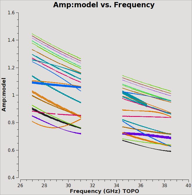
Inspecting the logger report shows that 3C147 has a flux density ranging from ~1.0-1.47 Jy across all spws.
We can plot the model data using plotms (Figure 1):
# In CASA
plotms(vis='G192-BP.ms', field='0', antenna='ea03', \
       xaxis='freq', yaxis='amp', ydatacolumn='model',coloraxis='ant2')
This plot shows baselines to antenna ea03. Since we provided both a spectral and a spatial model for this well resolved calibrator, each baseline has a somewhat different behavior.
Calibrating delays and initial bandpass solutions
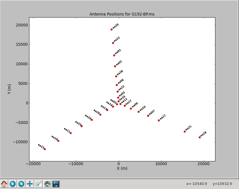
As a first step, we need to specify a reference antenna for all phase calibrations. It is desirable to use an antenna that is near the center of the array and that has a minimum of flags. The array can be mapped with plotants:
# In CASA: plotting antenna locations
plotants(vis='G192-BP.ms')
Although the plot is a bit crowded (Figure 2), a zoom in (the icon with the magnifying glass) shows that ea05 sits close to the center and appears to be a good choice.
We start with a phase-only calibration solution on a narrow range of channels near the center of each spectral window on the bandpass calibrator 3C84 to flatten them with respect to time before solving for the bandpass. This will remove most of the decorrelation of the signal. The range 60~68 should work, and we derive a solution for each individual integration:
# In CASA: phase only calibration
gaincal(vis='G192-BP.ms', caltable='calG192.G0', \
        field='1', spw='*:60~68', \
        gaintype='G', refant='ea05', calmode='p', \
        solint='int', minsnr=3)
- refant='ea05' : Use ea05 as the reference antenna
- solint='int' : Do a per-integration solve (every 6 seconds, since we've time-averaged the data).
- minsnr=3 : Apply a minimum signal-to-noise cutoff. Solutions with less than this value will be flagged.
- gaintable is not set here as we have already applied pre-calibrations.
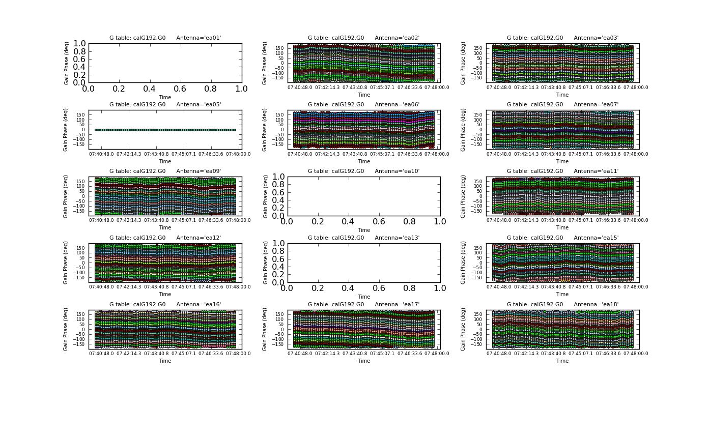
Plot the phase solutions (using full phase range, -180 to 180, instead of autorange):
# In CASA
plotcal(caltable='calG192.G0', xaxis='time', yaxis='phase', \
        iteration='antenna', plotrange=[-1,-1,-180,180])
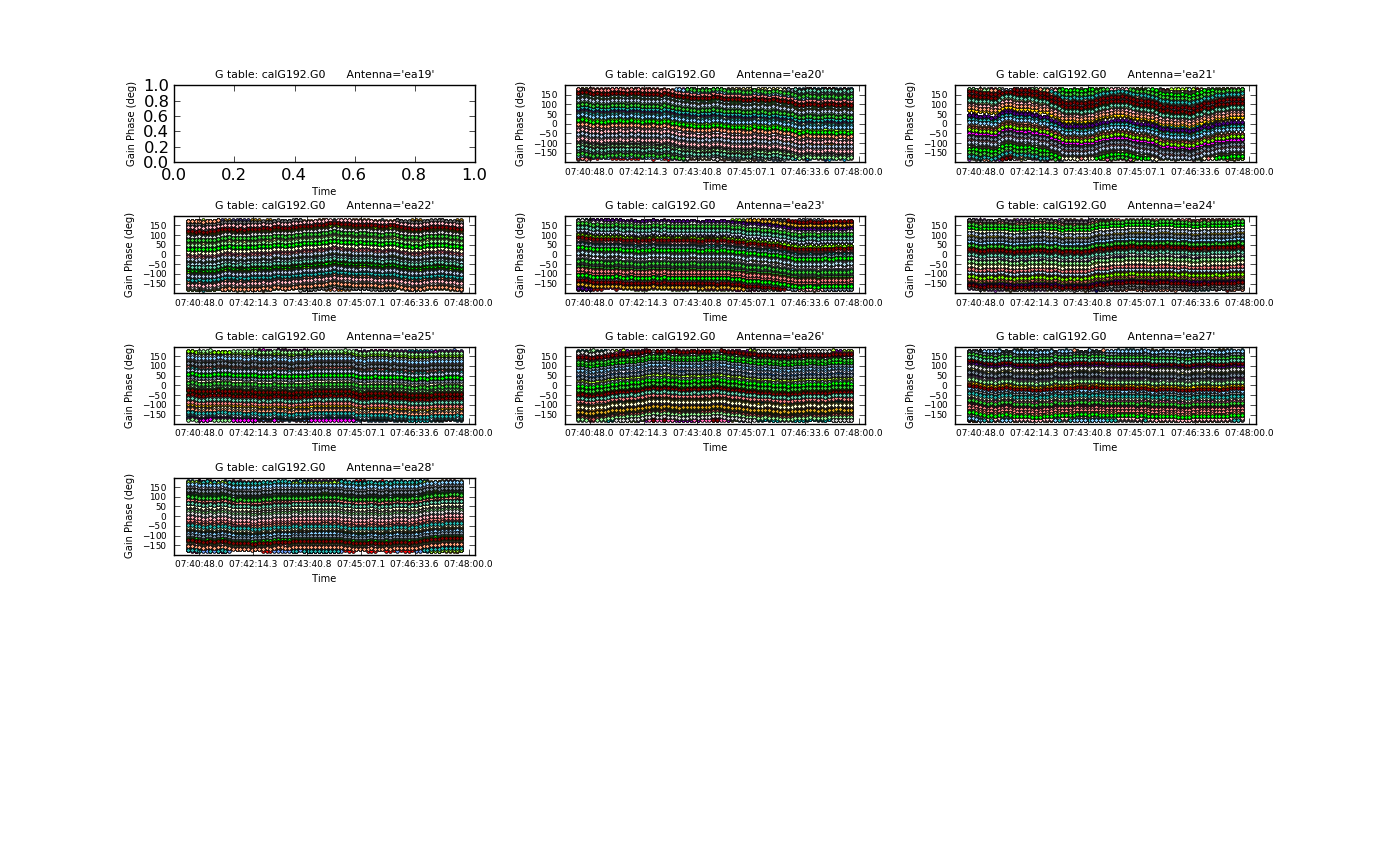
Plot the phase solutions. We will produce multipanel plots and write to output files (Figures 3a & 3b). The output files generated are PNG files and can be viewed within CASA by executing an external viewer program, e.g., !xv plotG192_plotcal_G0p1.png; or by running any number of image viewing applications such as xv, Preview, Gimp, Photoshop, etc., external to CASA at the OS level. (Note that the hardcopy only shows the first page):
# In CASA
plotcal(caltable='calG192.G0', xaxis='time', yaxis='phase', \
        antenna='0~10,12~15', subplot=531, iteration='antenna', \
        plotrange=[-1,-1,-180,180], fontsize=8.0, \
        markersize=3.0, figfile='plotG192_plotcal_G0p1.png')
plotcal(caltable='calG192.G0', xaxis='time', yaxis='phase', \
        antenna='16~26', subplot=531, iteration='antenna', \
        plotrange=[-1,-1,-180,180], fontsize=8.0, \
        markersize=3.0, figfile='plotG192_plotcal_G0p2.png')
We can now solve for the residual delays using the gaintype='K' option in gaincal. Note that this currently does not do a global fringe-fitting solution for delays, but instead does a baseline-based delay solution per spw for all baselines to the reference antenna, treating these as antenna-based delays. In most cases, with high enough S/N to get baseline-based delay solutions, this will suffice. We avoid the edge channels of each spectral window by selecting channels 5~122:
# In CASA: residual delays
gaincal(vis='G192-BP.ms', caltable='calG192.K0', \
        field='1', spw='*:5~122', gaintype='K', \
        gaintable=['calG192.G0'],
        refant='ea05', solint='inf', minsnr=3)
Note that we have also pre-applied our initial phase table calG192.G0.
Alternatively, you can also derive a delay across all spws of a baseband. If this is desired, use combine='spw' in gaincal and run the task for each baseband separately. The solutions from the second and following runs can be appended to the same calibration table via append=T.
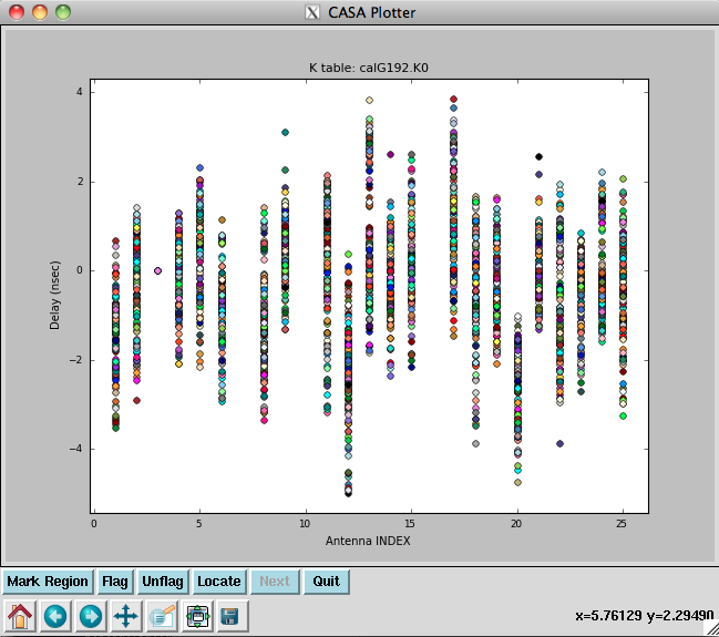
Now plot the delays, in nanoseconds, as a function of antenna index (you will get one for each spw and polarization):
# In CASA
plotcal(caltable='calG192.K0', xaxis='antenna', yaxis='delay')
The delays range from around -5 to 4 nanoseconds (Figure 4).
Now solve for the antenna bandpasses using the previously generated tables calG192.G0 and calG192.K0:
# In CASA: antenna bandpasses
bandpass(vis='G192-BP.ms', caltable='calG192.B0', \
         gaintable=['calG192.G0', 'calG192.K0'], \
         field='1', refant='ea05', solnorm=False, \
         bandtype='B', solint='inf')
WARNING: You must set solnorm=False here or later on you will find some offsets among spws due to the way the amplitude scaling adjusts weights internally during solving.
You will see, in the terminal window, some reports of solutions failing due to "Insufficient unflagged antennas"—note that these are for bad channels that have been pre-flagged.
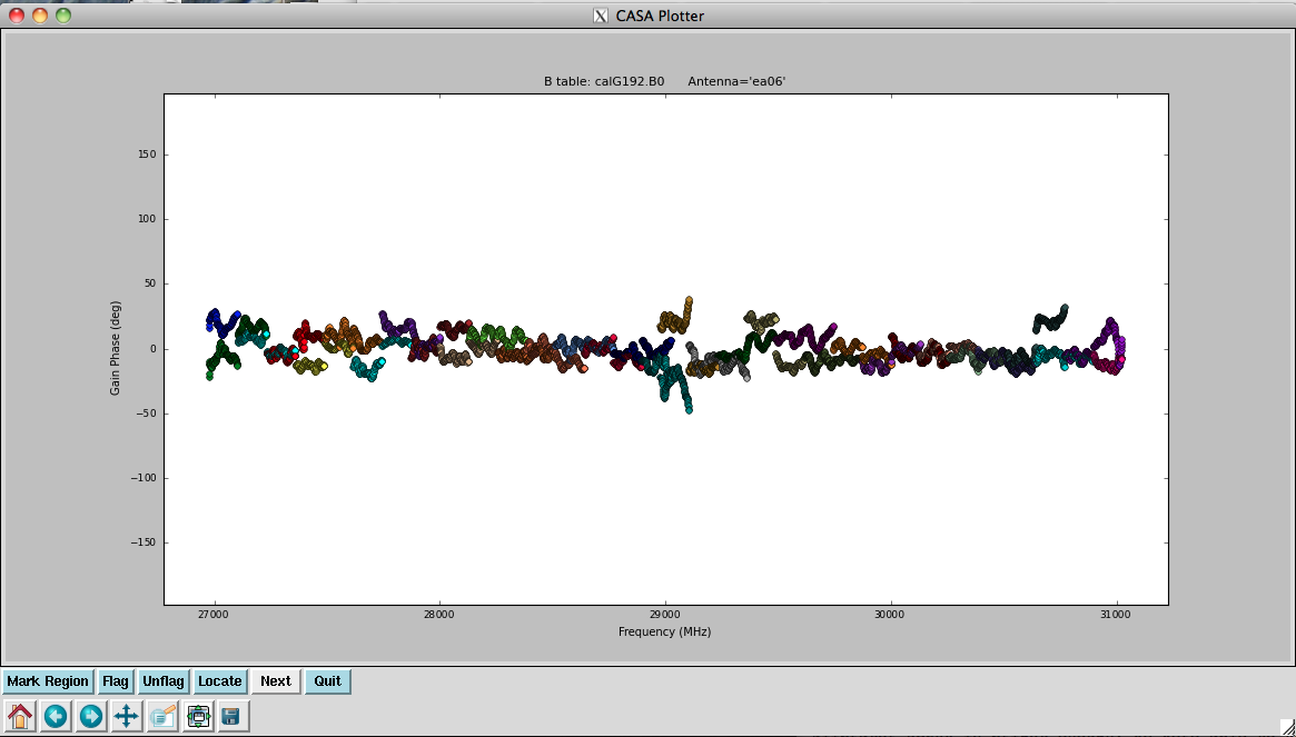
Plot the resulting bandpasses in amplitude and phase. Note that the first panel with ea01 is empty as it is completely flagged. Proceed to ea06 to see the plots as shown in Figures 5a, 5b, 6a, and 6b:
# In CASA
plotcal(caltable='calG192.B0', xaxis='freq', yaxis='amp', \
        spw='0~31', iteration='antenna')
#
plotcal(caltable='calG192.B0', xaxis='freq', yaxis='amp', \
        spw='32~63', iteration='antenna')
#
plotcal(caltable='calG192.B0', xaxis='freq', yaxis='phase', \
        iteration='antenna', spw='0~31', \
        plotrange=[-1,-1,-180,180])
#
plotcal(caltable='calG192.B0', xaxis='freq', yaxis='phase', \
        iteration='antenna', spw='32~63', \
        plotrange=[-1,-1,-180,180])
Bootstrapping the bandpass calibrator spectrum
Since there is no a priori spectral information for our chosen bandpass calibrator—3C84—we need to bootstrap to find its spectral index, then recalibrate with this information in order to avoid folding the intrinsic spectral shape of 3C84 into our calibration.
First, we again do a phase-only calibration solution, this time for both the bandpass and the flux density calibrator. This will correct for decorrelation of the signals. Again we use the channel range 60~68 and apply the bandpass and delay calibration tables:
# In CASA: flux and bandpass calibrators gain
gaincal(vis='G192-BP.ms', caltable='calG192.G1p', field='0,1', \
        gaintable=['calG192.K0', 'calG192.B0'], \
        gaintype='G', refant='ea05', calmode='p', solint='int', minsnr=3)
Now we are ready to solve for both, phase and gain for each scan:
# In CASA: flux and bandpass calibrators gain
gaincal(vis='G192-BP.ms', caltable='calG192.G1', field='0,1', \
        gaintable=['calG192.K0', 'calG192.B0','calG192.G1p'], \
        gaintype='G', refant='ea05', calmode='ap', solint='inf', minsnr=3)
With gain solutions for the flux density and bandpass calibrators, we can now use fluxscale to scale the gain amplitudes of the bandpass calibrator using those of the flux density calibrator:
# In CASA: bandpass calibrator gain amplitudes scaling
flux1 = fluxscale(vis='G192-BP.ms', caltable='calG192.G1', \
                  fluxtable='calG192.F1', reference='0', \
                  transfer='1', listfile='3C84.fluxinfo', fitorder=1)
- flux1 = fluxscale(...): we allow fluxscale to use the variable flux1 for the output Python dictionary that is returned, which has information about the flux scaling. You can inspect the output dictionary flux1 by typing "print flux1" at the CASA command line.
- fluxtable='calG192.F1': this is the output scaled gain table. Since we are only using this to find the spectral index of 3C84, we won't be using this table.
- listfile='3C84.fluxinfo': an output file that contains the derived flux values and fit information.
- fitorder=1: only find a spectral index, ignoring curvature in the spectrum.
- reference='0': the reference field from which the flux scaling is transferred (here: the flux calibrator 3C147, field 0)
- transfer='1': the target field to which the flux scaling is transferred (here: the bandpass calibrator 3C84, field 1)
The last line in the file (and displayed in the logger) shows:
Fitted spectrum for 3c84-J0319+413 with fitorder=1: Flux density = 29.0282 +/- 0.0308648 (freq=32.5128 GHz) spidx=-0.538758 +/- 0.00882913
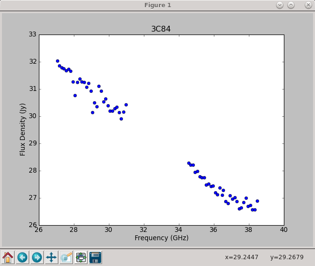
Using the information in the returned flux1 dictionary, we can plot the derived spectrum (Figure 7):
# In CASA
freq = flux1['freq'] / 1e9
spw_list = range(0,64)
spw_str = []
for i in spw_list:
   thisspw = str(i)
   spw_str.append(thisspw)
# In CASA
bootstrapped_fluxes = []
for j in spw_str:
    thisflux = flux1['1'][j]['fluxd'][0]
    if thisflux ==None:
        continue
    else:
        bootstrapped_fluxes.append(thisflux)
# In CASA - this section creates the plot seen in Figure 7
pl.clf()
pl.plot(freq, bootstrapped_fluxes, 'bo')
pl.xlabel('Frequency (GHz)')
pl.ylabel('Flux Density (Jy)')
pl.title('3C84')
pl.show()
We can use the model from fluxscale to fill the MODEL column with 3C84's spectral information using setjy. With standard='fluxscale', we can directly use the flux1 Python dictionary as input via fluxdict:
# In CASA: spectral information
setjy(vis='G192-BP.ms', field='1', scalebychan=True, \
      standard = 'fluxscale', fluxdict=flux1)
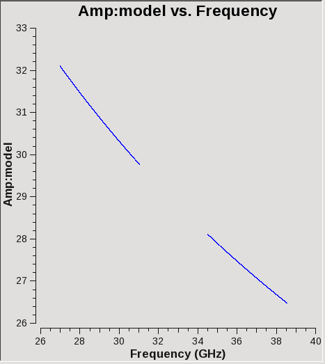
Checking with plotms that the data have been appropriately filled (Figure 8):
# In CASA
plotms(vis='G192-BP.ms', field='1', antenna='ea05&ea02', \
       xaxis='freq', yaxis='amp', ydatacolumn='model')
We redo the previous calibration using this new model information. Although the commands are the same as what we issued earlier, keep in mind that the model values for the bandpass calibrator have changed, and therefore the results of these calibration calculations will differ:
# In CASA: phase only recalibration
gaincal(vis='G192-BP.ms', caltable='calG192.G0.b', \
        field='1', spw='*:60~68', \
        gaintype='G', refant='ea05', calmode='p', \
        solint='int', minsnr=3)
# In CASA: residual delays recalibration
gaincal(vis='G192-BP.ms', caltable='calG192.K0.b', \
        gaintable=['calG192.G0.b'], \
        field='1', spw='*:5~122', gaintype='K', \
        refant='ea05', solint='inf', minsnr=3)
# In CASA: antenna bandpasses recalibration
bandpass(vis='G192-BP.ms', caltable='calG192.B0.b', \
         gaintable=['calG192.G0.b', 'calG192.K0.b'], \
         field='1', refant='ea05', solnorm=False, \
         bandtype='B', solint='inf')
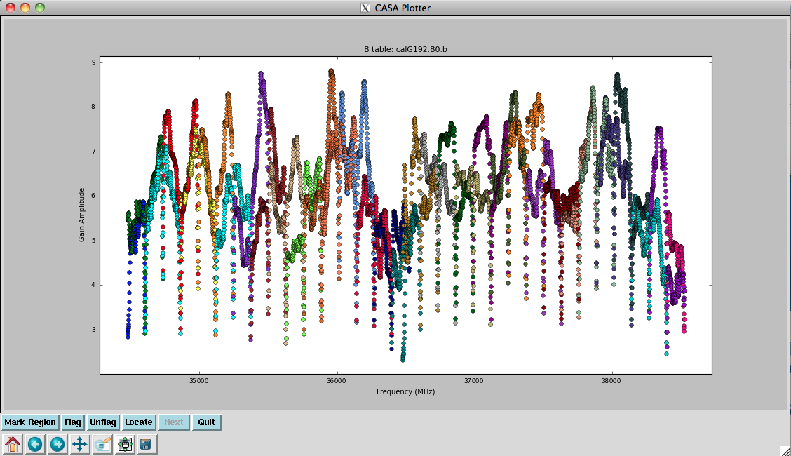
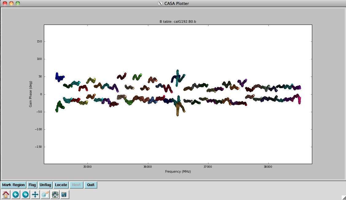
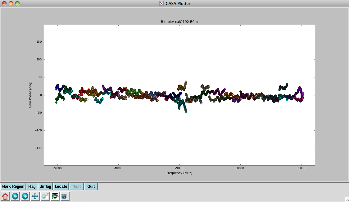
Finally we inspect these solutions (Figures 9a, 9b, 10a, and 10b):
# In CASA - Figure 9a
plotcal(caltable='calG192.B0.b', xaxis='freq', yaxis='amp', \
        spw='0~31', iteration='antenna')
# Figure 9b
plotcal(caltable='calG192.B0.b', xaxis='freq', yaxis='amp', \
        spw='32~63', iteration='antenna')
# Figure 10a
plotcal(caltable='calG192.B0.b', xaxis='freq', yaxis='phase', \
        iteration='antenna', spw='0~31', \
        plotrange=[-1,-1,-180,180])
# Figure 10b
plotcal(caltable='calG192.B0.b', xaxis='freq', yaxis='phase', \
        iteration='antenna', spw='32~63', \
        plotrange=[-1,-1,-180,180])
They look virtually unchanged from the previous solutions, with the exception that the amplitude scaling is corrected for the spectrum of 3C84. Now that we have the final version of our delay and bandpass calibration tables, calG192.K0.b and calG192.B0.b can be used for all subsequent calibration steps.
Last checked on CASA Version 4.5.2


