Plotmosaic
From CASA Guides
Return to Analysis Utilities
This page documents the plotmosaic function of Python module analysisUtils.
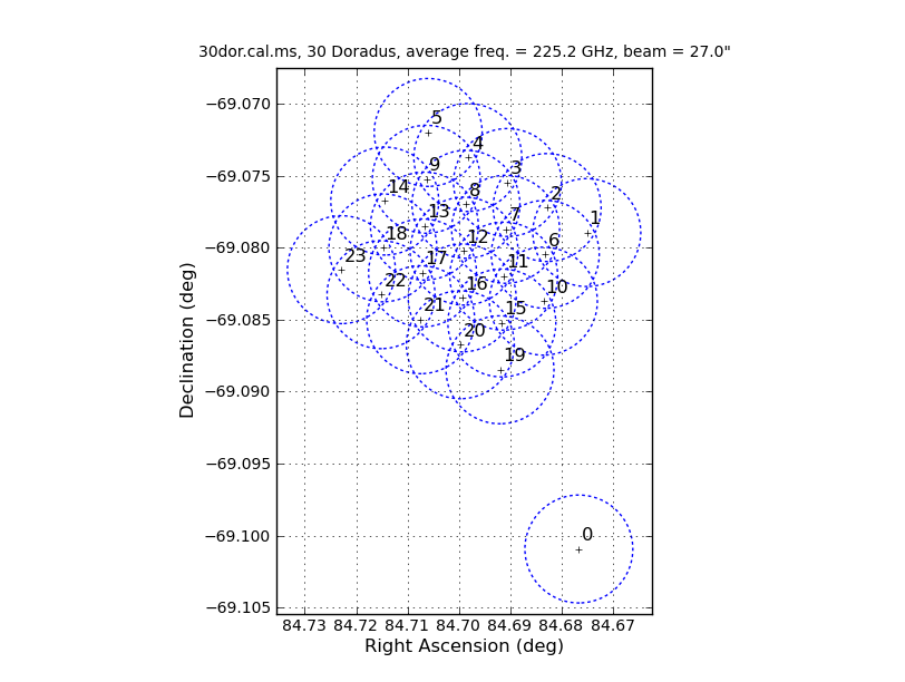
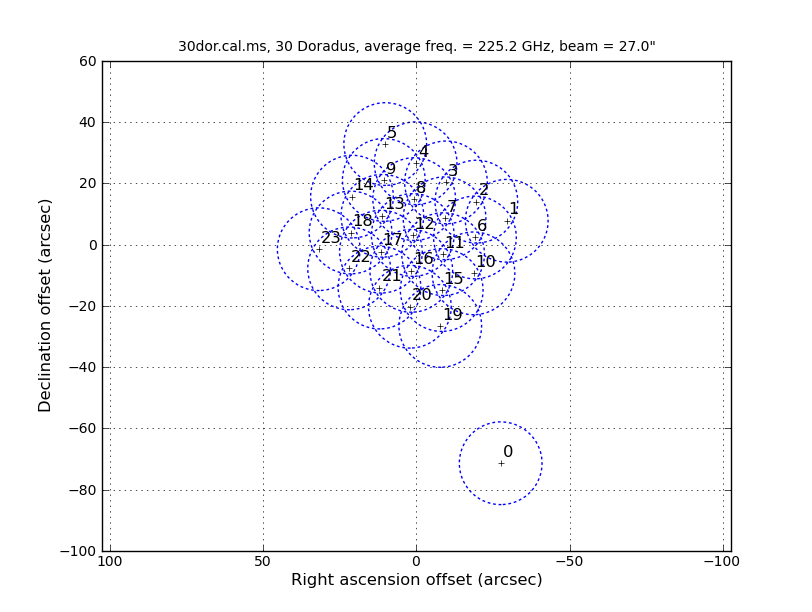
This function produces a plot of the pointings in a MS with primary beam FWHM circles and field names overlaid. For a multi-source file, you can include the sourceid to limit the fields to the science target. The default coordinate system is 'relative'. You can also use 'absolute', in which case the RA and Dec are shown in decimal degrees. This could be improved to be HH:MM:SS if there is demand. (Note: plotmosaic and plotMosaic are synonyms.)
Usage:
au.plotmosaic(vis, sourceid=2, figfile='mosaic.png', coord='relative', skipsource=-1, doplot=True, help=False, sciencespws=False, vm=)
Notes:
- The sourceid may be either an integer, integer string, or the string name of the source (but it cannot be a list).
- If doplot=False, then the central field ID is returned as an integer. Otherwise, a list is returned which is useful for determining the required image size for clean: [centralField, maxRA, minRA, minDec, maxDec] where the angles are in units of arcsec relative to the center.
- If coord='absolute', then nothing is returned.
- figfile can be either a string or "True". In the latter case, the automatic name will be: [vis].pointings.[coord].png
- The title will include the visibility file name but with any parent directory removed.
- If sciencespws=True, then run ValueMapping to determine science spws.
- If vm is not , then it's assumed to be a ValueMapping structure.
- The size of the circle plotted is 1.17*lambda/dish_diameter, which is correct for ALMA antennas
Examples
# In CASA
CASA <2>: au.plotMosaic("30dor.cal.ms",sourceid='30 Doradus',doplot=False)
Field IDs with matching source ID =  [ 0  1  2  3  4  5  6  7  8  9 10 11 12 13 14 15 16 17 18 19 20 21 22 23]
Got longitude = -67.755 deg
Mean frequency = 225.180484 GHz
Found 24 pointings
Field 12 is closest to the center of the area covered (3.3 arcsec away).
  Out[18]: 12
# In CASA
CASA <3>: au.plotMosaic("30dor.cal.ms",sourceid='30 Doradus',coord='abs',figfile='/tmp/absolute.png')
Field IDs with matching source ID =  [ 0  1  2  3  4  5  6  7  8  9 10 11 12 13 14 15 16 17 18 19 20 21 22 23]
Got longitude = -67.755 deg
Mean frequency = 225.180484 GHz
Found 24 pointings
Field 12 is closest to the center of the area covered (3.3 arcsec away).
Wrote file = /tmp/absolute.png
# In CASA
CASA <4>: au.plotMosaic("30dor.cal.ms",sourceid='30 Doradus',coord='rel',figfile='/tmp/relative.png')
Field IDs with matching source ID =  [ 0  1  2  3  4  5  6  7  8  9 10 11 12 13 14 15 16 17 18 19 20 21 22 23]
Got longitude = -67.755 deg
Mean frequency = 225.180484 GHz
Found 24 pointings
Field 12 is closest to the center of the area covered (3.3 arcsec away).
Wrote file = /tmp/relative.png
  Out[4]:
[12,
 58.898348082265692,
 -56.505271415428538,
 59.801877597487355,
 -98.429477166421918]

