M100 Band3 Combine 4.2.2
Overview
Combine and Image the 7m+12m
Split off CO spws
# In CASA
os.system('m100_*m.ms.listobs')
listobs('M100_Band3_12m_CalibratedData.ms',listfile='m100_12m.ms.listobs')
listobs('M100_Band3_7m_CalibratedData.ms',listfile='m100_7m.ms.listobs')
Below are the observation and spectral window tables from the listobs.
12m data:

ObservationID = 0         ArrayID = 0
  Date        Timerange (UTC)          Scan  FldId FieldName             nRows     SpwIds   Average Interval(s)
  10-Sep-2011/18:28:43.4 - 18:41:00.4    11      1 M100                      1320  [0, 1, 2, 3]  [6.05, 6.05, 6.05, 6.05]

Spectral Windows:  (4 unique spectral windows and 1 unique polarization setups)
  SpwID  Name   #Chans   Frame   Ch1(MHz)  ChanWid(kHz)  TotBW(kHz) BBC Num  Corrs
  0              3840   TOPO  113726.419       488.281   1875000.0       1  XX  YY
  1              3840   TOPO  111851.419       488.281   1875000.0       2  XX  YY
  2              3840   TOPO  103663.431      -488.281   1875000.0       3  XX  YY
  3              3840   TOPO  101850.931      -488.281   1875000.0       4  XX  YY

7m data:

ObservationID = 0         ArrayID = 0
  Date        Timerange (UTC)          Scan  FldId FieldName             nRows     SpwIds   Average Interval(s)
  17-Mar-2013/04:44:04.3 - 04:50:43.7    11      1 M100                       168  [0, 1]  [10.1, 10.1]

Spectral Windows:  (4 unique spectral windows and 1 unique polarization setups)
  SpwID  Name                           #Chans   Frame   Ch1(MHz)  ChanWid(kHz)  TotBW(kHz) BBC Num  Corrs
  0      ALMA_RB_03#BB_3#SW-01#FULL_RES   4080   TOPO  111811.300       488.281   1992187.5       3  XX  YY
  1      ALMA_RB_03#BB_4#SW-01#FULL_RES   4080   TOPO  113686.300       488.281   1992187.5       4  XX  YY
  2      ALMA_RB_03#BB_1#SW-01#FULL_RES   4080   TOPO  111798.250       488.281   1992187.5       1  XX  YY
  3      ALMA_RB_03#BB_2#SW-01#FULL_RES   4080   TOPO  113673.250       488.281   1992187.5       2  XX  YY
Examination of the listobs files shows that the CO is spw=0 for the 12m data and in spws='1,3' for the 7m data. The 12m data has 48 fields and the 7m has 24 fields. There are two for the 7m data because some of the data was taken with a slightly different correlator setup.
Also note that the integration time per visibility (average interval parameter in listobs) is different: 6.05s for the 12m data and 10.1s for the 7m. This will be important to know later in order to correctly weight the combined data.
# In CASA
os.system('rm -rf m100_12m_CO.ms')
split(vis='M100_Band3_12m_CalibratedData.ms',
      outputvis='m100_12m_CO.ms',spw='0',field='M100',
      datacolumn='data',keepflags=False)
os.system('rm -rf m100_7m_CO.ms')
split(vis='M100_Band3_7m_CalibratedData.ms',
      outputvis='m100_7m_CO.ms',spw='1,3',field='M100',
      datacolumn='data',keepflags=False)
Because the continuum is too weak to contribute to a 5km/s channel we will forgo the the continuum subtraction step.
Concat with 1/sigma2 scaling of Weights
<figure id="7m_WT.png">

</figure>
<figure id="12m_WT.png">

</figure>
When combining data with disparate properties it is very important that the relative weights of each visibility be in the correct proportion to the other data according to the radiometer equation. Formally, the visibility weights should be proportional to 1/sigma**2 where sigma is the variance or rms noise of a given visibility.
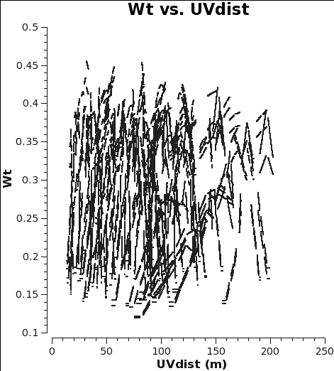
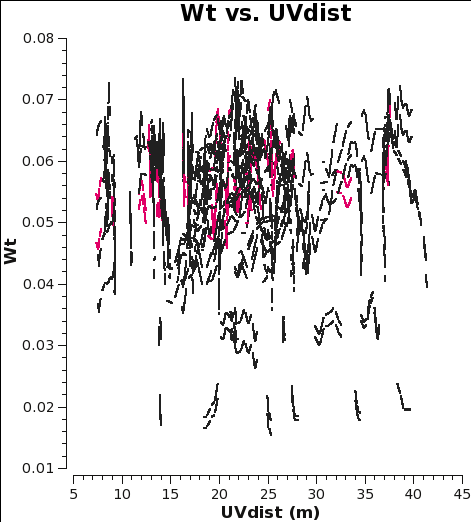
CASA currently scales the weights by 1/[(Tsys(i) * Tsys(j)] if calwt=True for the Tsys table applycal. To verify, we plot the weights of the 7m and 12m data. No averaging can be turned on when plotting the weights.
# In CASA
os.system('rm -rf 7m_WT.png 12m_WT.png')
plotms(vis='m100_12m_CO.ms',yaxis='wt',xaxis='uvdist',spw='0~2:200',
       coloraxis='spw',plotfile='12m_WT.png')
#
plotms(vis='m100_7m_CO.ms',yaxis='wt',xaxis='uvdist',spw='0~2:200',
       coloraxis='spw',plotfile='7m_WT.png')
As you can see from these plots, the weights are quite similar at this stage because the data were taken under similar weather conditions and hence Tsys.
Assuming that the 7m and 12m antennas have similar apperture and quantization efficiencies (a reasonable assumption since they were designed this way), the rms noise in a single channel for a single visibility is:
[math]\displaystyle{ \sigma_{ij}=\frac{2k}{A_{eff}} }[/math] [math]\displaystyle{ \sqrt{\frac{T_{sys,i} T_{sys,j}}{\Delta\nu_{ch} t_{ij}}} }[/math]
<figure id="Intcombo_0.193_WT.png">

</figure>
Where k is Boltzmann's constant, Aeff is the effective antenna area, Tsys,i is the system temperature for antenna i, Δνch is the channel width, and tij is the integration time per visibility.
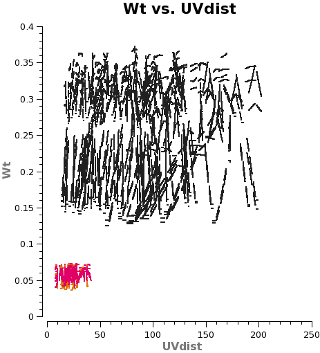
The two key things that are different between the 7m and 12m-array data are that the effective dish Areas are different by (7/12)2 and the integration times are different by sqrt(10.1/6.05). Since dish area is in the numerator of the radiometer equation and integration time per visibility is in the denominator, and assuming WT propto 1/sigma2, the 7m weight should be scaled by: (7./12.)4 x (10.1/6.05) = 0.193 to account for the difference in telescope size and integration time per visibility.
# In CASA
# Concat and scale weights
os.system('rm -rf M100_Intcombo_0.193.ms')
concat(vis=['m100_12m_CO.ms','m100_7m_CO.ms'],
       concatvis='M100_Intcombo_0.193.ms',
       visweightscale=[1,0.193])
Now plot the concatenated weights to verify they are as expected.
# In CASA
os.system('rm -rf Intcombo_0.193_WT.png')
plotms(vis='M100_Intcombo_0.193.ms',yaxis='wt',xaxis='uvdist',spw='0~2:200',
       coloraxis='spw',plotfile='Intcombo_0.193_WT.png')
<figure id="M100_Intcombo_0.193_vel.png">

</figure>
Some additional useful plots of the combined data (Let each plot finish before cutting and pasting next plot. If plotms gui disappears, exit CASA and restart):
amplitude as a function of uv-distance
# In CASA
os.system('rm -rf M100_Intcombo_0.193 _uvdist.png')
plotms(vis='M100_Intcombo_0.193.ms',yaxis='amp',xaxis='uvdist',spw='',
       avgchannel='5000',
       coloraxis='spw',plotfile='M100_Intcombo_0.193_uvdist.png')
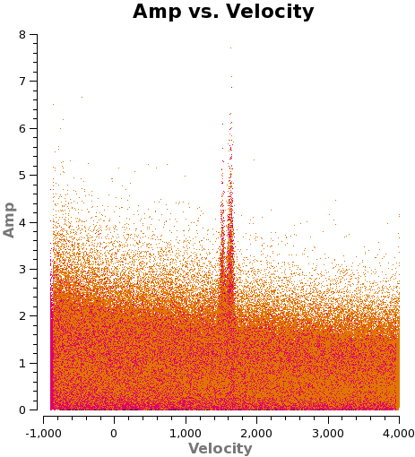
The CO line as a function of velocity (note this plot takes a while).
# In CASA
os.system('rm -rf M100_Intcombo_0.193_vel.png')
plotms(vis='M100_Intcombo_0.193.ms',yaxis='amp',xaxis='velocity',spw='',
       avgtime='1e8',avgscan=True,coloraxis='spw',avgchannel='5',
       transform=True,freqframe='LSRK',restfreq='115.271201800GHz',
       plotfile='M100_Intcombo_0.193_vel.png')
To see each spectral window independently, run the command again but remove plotfile, and add iteraxis='spw'.
Image Using Automasking Technique
The commands in this section attempt to do an iterative automasking procedure down to a user specified threshold=stop*rms where stop is typically 2-3. It takes some care to ensure that the generated masks (i) only have values of 0 or 1; (ii) are themselves masked at the minpb level. It also removes very small masked regions that are consistent with noise bumps using a function in scipy. A typical setting is to remove mask regions that are 1/2 the beam area in pixels.
The commands have been split into multiple sections to aid cut and paste -- do them one at a time. If you stop CASA and restart you will need to cut and paste again from the Define Parameters section on down.
Define Parameters
# In CASA

### Initialize
import scipy.ndimage

### Define clean parameters
vis='M100_Intcombo_0.193.ms'
prename='M100_Intcombo_0.193_cube'
myimage=prename+'.image'
myflux=prename+'.flux'
mymask=prename+'.mask'
myresidual=prename+'.residual'
imsize=800
cell='0.5arcsec'
minpb=0.2
restfreq='115.271201800GHz'
outframe='LSRK'
spw='0~2'
width='5km/s'
start='1400km/s'
nchan=70
robust=0.5
phasecenter='J2000 12h22m54.9 +15d49m10'
scales=[0]
smallscalebias=0.6

### Setup stopping criteria with multiplier for rms.

stop=3.

### Minimum size multiplier for beam area for removing very small mask regions.

pixelmin=0.5
Make Initial Dirty Image and find rms noise
# In CASA
### Make initial dirty image
os.system('rm -rf '+prename+'.* ' +prename+'_*')
clean(vis=vis,imagename=prename,
      imagermode='mosaic',ftmachine='mosaic',minpb=minpb,
      imsize=imsize,cell=cell,spw=spw,
      weighting='briggs',robust=robust,phasecenter=phasecenter,
      mode='velocity',width=width,start=start,nchan=nchan,
      restfreq=restfreq,outframe=outframe,veltype='radio',
      mask='',
      niter=0,interactive=F)
Find properties of the dirty image
Find the peak in the dirty cube.
# In CASA
myimage=prename+'.image'
bigstat=imstat(imagename=myimage)
peak= bigstat['max'][0]
print 'peak in cube = '+str(peak)
### Sets threshold of first loop, try 2-4. Subsequent loops are set thresh/2
thresh = peak /4.
Find the rms noise in the dirty cube or set it by hand (can be useful for dynamic range limited emission).
# In CASA
### If True: find the rms in two line-free channels; If False:  Set rms by hand in else statement.
if True:
    chanstat=imstat(imagename=myimage,chans='4')
    rms1= chanstat['rms'][0]
    chanstat=imstat(imagename=myimage,chans='66')
    rms2= chanstat['rms'][0]
    rms=0.5*(rms1+rms2)
else:
    rms=0.013

# print rms
print 'rms in a channel = '+str(rms)
Define minimum size of masked region
# In CASA
# Deterimine the beam area in pixels for later removal of very small
# mask regions
major=imhead(imagename=myimage,mode='get',hdkey='beammajor')['value']
minor=imhead(imagename=myimage,mode='get',hdkey='beamminor')['value']
pixelsize=float(cell.split('arcsec')[0])
beamarea=(major*minor*pi/(4*log(2)))/(pixelsize**2)
print 'beamarea in pixels =', beamarea
Automasking Loop
# In CASA
n=-1
while (thresh >= stop*rms):
    n=n+1
    print 'clean threshold this loop is', thresh
    threshmask = prename+'_threshmask' +str(n)
    maskim = prename+'_fullmask' +str(n)
    immath(imagename = [myresidual],
           outfile = threshmask,
           expr = 'iif(IM0 > '+str(thresh) +',1.0,0.0)',
           mask=myflux+'>'+str(minpb))
    if (n==0):
        os.system('cp -r '+threshmask+' '+maskim+'.pb')
        print 'This is the first loop'
    else:
        makemask(mode='copy',inpimage=myimage,
                 inpmask=[threshmask,mymask],
                 output=maskim)
        imsubimage(imagename=maskim, mask=myflux+'>'+str(minpb),
                   outfile=maskim+'.pb')
    print 'Combined mask ' +maskim+' generated.'

    # Remove small masks
    os.system('cp -r '+maskim+'.pb ' +maskim+'.pb.min')
    maskfile=maskim+'.pb.min'
    ia.open(maskfile)
    mask=ia.getchunk()
    labeled,j=scipy.ndimage.label(mask)
    myhistogram = scipy.ndimage.measurements.histogram(labeled,0,j+1,j+1)
    object_slices = scipy.ndimage.find_objects(labeled)
    threshold=beamarea*pixelmin
    for i in range(j):
        if myhistogram[i+1]<threshold:
            mask[object_slices[i]] = 0


    ia.putchunk(mask)
    ia.done()
    print 'Small masks removed and ' +maskim +'.pb.min generated.'

    os.system('rm -rf '+mymask+'')
    clean(vis=vis,imagename=prename,
          imagermode='mosaic',ftmachine='mosaic',minpb=minpb,
          imsize=imsize,cell=cell,spw=spw,
          weighting='briggs',robust=robust,phasecenter=phasecenter,
          mode='velocity',width=width,start=start,nchan=nchan,
          restfreq=restfreq,outframe=outframe,veltype='radio',
          mask = maskim+'.pb.min',
          multiscale=scales,smallscalebias=smallscalebias,
          interactive = F,
          niter = 10000,
          threshold = str(thresh) +'Jy/beam')


    if thresh==stop*rms: break
    thresh = thresh/2.
    # Run a final time with stop*rms if more than a little above
    # stop*rms. Also make a back-up of next to last image
    if (thresh < stop*rms and thresh*2.>1.05*stop*rms):
        thresh=stop*rms
        os.system('cp -r '+myimage+' '+myimage+str(n))