What is CASA?
A brief summary of the CASA package.
The Basics
CASA (Common Astronomy Software Applications) is the data analysis software package for the next generation of radio telescopes, specifically ALMA and the EVLA. It can also be used to process archival and current VLA data. CASA performs end-to-end processing of the large datasets resulting from these new telescopes: from data calibration to image analysis. Detailed information is available in the CASA Cookbook, which you can download from here. The package is still under development, and full functionality is not yet available. Check with the CASA homepage to find out the latest status of the project.
Data Storage
CASA stores data in a Measurement Set (MS). Logically, it is a generalized description of data from any interferometer or single-dish telescope. Physically, it is several tables in a directory on disk. Tables in CASA are actually directories containing files that are sub-tables. If you create a MS called 'AM675.ms', the sub-tables are stored in the directory AM675.ms/. Calibration solutions or images will also be written to disk as directories and sub-directories.
The MAIN data table is arranged so that each row is a single timestamp for a single spectral window and a single baseline. There are several columns. DATA holds the original visibility data, CORRECTED holds the calibrated data, MODEL holds the Fourier inversion of a particular model image, and IMAGING_WEIGHT holds the weights to be used in imaging. Occasionally, you will need to specify a column for a particular task, so it is useful to know about them.
End-to-end
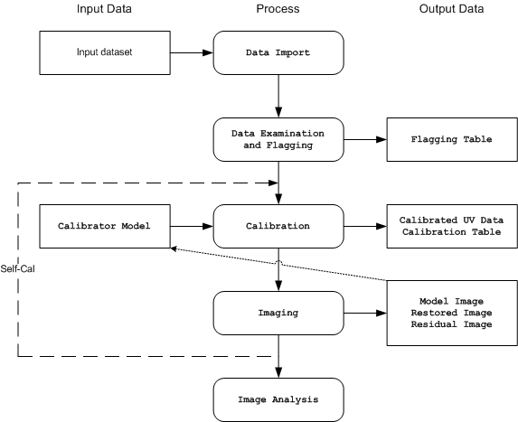
An overview of the process from Loading to Imaging:
Importing Data and Images:
Data is initially loaded into CASA using one of three import tasks:
These import UVFITS, VLA and EVLA/ALMA data, respectively. Two other related tasks are available:
- importfits: can be used to import a FITS image into a CASA image format table;
- concat: can be used to concatenate a second measurement set into a given MS.
Examing, Editing and Flagging
There are several tasks to list, plot and/or flag data in a MS:
- listobs: summarizes the contents of a MS;
- flagmanager: saves and manages versions of the flagging entries in the MS;
- flagautocorr: non-interactively flags auto-correlations;
- plotms: interactively plots and flags visibility data in 2-D;
- flagdata: non-interactively flags and unflags specified data;
- viewer: displays MS data, with some editing capabilities.
Calibration
During calibration, the user specifies a set of calibrations to pre-apply before solving for a particular effect (gain or bandpass or polarization). The user (not the task!) specifies a calibration table to store the solutions. Take care in naming the table for future use. Finally, the calibration is applied to the dataset, and calibrated data are written into the CORRECTED column.
Calibration tasks are:
- setjy: computes the model visibilities for a specified source given a flux density. setjy 'knows' about standard calibrator sources;
- bandpass: solves for frequency-dependent complex gains;
- gaincal: solves for time-dependent complex gains;
- fluxscale: bootstraps the flux density scale from standard calibrators;
- polcal: polarization calibration;
- accum: accumulates incremental calibration solutions into a cumulative table;
- smoothcal: smooths calibration solutions derived from one or more sources;
- applycal: applies calculated calibration solutions;
- clearcal: re-initializes calibrated visibility data in a given MS;
- listcal: lists calibration solutions;
- plotcal: plots (and optionally flags) calibration solutions;
- uvcontsub: carry out uv-plane continuum subtraction for spectral-line data
- split: write out a new (calibrated) MS for specified sources
Imaging
At some point you want to actually see the model of the sky you have created from your data. The main tasks involved are:
- clean: calculates a deconvolved image based on the visibility data;
- feather: combines a single dish and synthesis image in the Fourier plane;
- ft: Fourier transforms the model (or component list) and fills the MODEL column;
- deconvolve: deconvolves an input image from a provided PSF.
Analysis
Of course, you will want to measure things! Several tasks are available to help with this:
- imhead: summarize and manipulate the 'header' information in a CASA image;
- imcontsub: perform continuum subtraction on a spectral-line image cube;
- immath: perform mathematical operations on or between images;
- immoments: compute the moments of an image cube;
- imstat: calculate statistics on an image or part of an image;
- imregrid: regrid an image onto the coordinate system of another image;
- viewer: there are useful statistics and plotting capabilities in the viewer.
Exporting
You can export your data from CASA using either exportuvfits or exportfits, which save the data in UVFITS or FITS formats, respectively.
Further Information
About CASA: The CASA Cookbook, available from the CASA homepage: [[1]] Other documentation is there as well.
About Interferometry: Synthesis Imaging in Radio Astronomy II (1999, ASP Conference Series Vol 180, eds. Taylor, Carilli and Perley)
About Python: see the vast internet. Googling 'Python manual' will turn up a number of options.
Please send any comments or questions about CASA to the NRAO helpdesk via your my.nrao.edu portal.
