Calibrating an EVLA OSRO HI data set
Overview
Currently, this describes the reduction of the Leo Ring dataset collected with WIDAR0. This page will need to be revised when "real" OSRO data is acquired.
Importing Data
importing data will probably be quirky; let's not discuss the details of this yet.
Get Some Basic Information on Your Data
Use listobs (roughly equivalent to LISTR in AIPS) to list information about your scans, correlator setup, and antenna positions.
#  listobs :: List data set summary in the logger
vis                 = 'leotest.ms'      #  Name of input visibility file (MS)
verbose             =       True
async               =      False        #  If true the taskname must be started using
                                        #   listobs(...)
will produce output that looks like this:
2010-02-11 18:11:34 INFO listobs	##########################################
2010-02-11 18:11:34 INFO listobs	##### Begin Task: listobs            #####
2010-02-11 18:11:34 INFO  	listobs::::casa
2010-02-11 18:11:34 INFO listobs	================================================================================
2010-02-11 18:11:34 INFO listobs	           MeasurementSet Name:  /export/home/rso-lchomiuk/test/Leo/leotest.ms      MS Version 2
2010-02-11 18:11:34 INFO listobs	================================================================================
2010-02-11 18:11:34 INFO listobs	   Observer: leo2pt     Project: T.B.D.
2010-02-11 18:11:34 INFO listobs	Observation: VLA
2010-02-11 18:11:34 INFO listobs	Data records: 70290       Total integration time = 11264.5 seconds
2010-02-11 18:11:34 INFO listobs	   Observed from   18-Dec-2009/10:52:17.0   to   18-Dec-2009/14:00:01.5 (UTC)
2010-02-11 18:11:35 INFO  	listobs::ms::summary
2010-02-11 18:11:35 INFO listobs	   ObservationID = 0         ArrayID = 0
2010-02-11 18:11:35 INFO listobs	  Date        Timerange (UTC)          Scan  FldId FieldName    nVis   Int(s)   SpwIds
2010-02-11 18:11:35 INFO listobs	  18-Dec-2009/10:52:17.0 - 10:53:45.0     1      0 J1042+1203   660    9.6      [0]
2010-02-11 18:11:35 INFO listobs	              10:54:14.0 - 10:56:51.5     2      1 J1042+1203   1122   9.71     [0]
2010-02-11 18:11:35 INFO listobs	              10:57:20.0 - 11:06:57.5     3      2 Leo-1        3894   9.92     [0]
2010-02-11 18:11:35 INFO listobs	              11:07:25.0 - 11:17:03.0     4      3 Leo-2        3894   9.93     [0]
2010-02-11 18:11:35 INFO listobs	              11:17:32.0 - 11:22:10.0     5      2 Leo-1        1914   9.86     [0]
2010-02-11 18:11:35 INFO listobs	              11:22:39.0 - 11:27:16.5     6      3 Leo-2        1914   9.83     [0]
2010-02-11 18:11:35 INFO listobs	              11:27:45.0 - 11:30:23.5     7      1 J1042+1203   1122   9.82     [0]
2010-02-11 18:11:35 INFO listobs	              11:30:52.0 - 11:40:30.0     8      2 Leo-1        3894   9.93     [0]
2010-02-11 18:11:35 INFO listobs	              11:40:59.0 - 11:50:36.5     9      3 Leo-2        3894   9.92     [0]
2010-02-11 18:11:35 INFO listobs	              11:51:05.0 - 11:55:42.5    10      2 Leo-1        1914   9.83     [0]
2010-02-11 18:11:35 INFO listobs	              11:56:11.0 - 12:00:49.0    11      3 Leo-2        1914   9.86     [0]
2010-02-11 18:11:35 INFO listobs	              12:01:18.0 - 12:03:56.0    12      1 J1042+1203   1122   9.76     [0]
2010-02-11 18:11:35 INFO listobs	              12:04:25.0 - 12:14:03.0    13      2 Leo-1        3894   9.93     [0]
2010-02-11 18:11:35 INFO listobs	              12:14:32.0 - 12:24:09.0    14      3 Leo-2        3894   9.9      [0]
2010-02-11 18:11:35 INFO listobs	              12:24:37.0 - 12:29:15.0    15      2 Leo-1        1914   9.86     [0]
2010-02-11 18:11:35 INFO listobs	              12:29:44.0 - 12:34:21.5    16      3 Leo-2        1914   9.83     [0]
2010-02-11 18:11:35 INFO listobs	              12:34:49.0 - 12:37:28.0    17      1 J1042+1203   1122   9.88     [0]
2010-02-11 18:11:35 INFO listobs	              12:37:57.0 - 12:47:35.0    18      2 Leo-1        3894   9.93     [0]
2010-02-11 18:11:35 INFO listobs	              12:48:04.0 - 12:57:41.5    19      3 Leo-2        3894   9.92     [0]
2010-02-11 18:11:35 INFO listobs	              12:58:10.0 - 13:02:48.0    20      2 Leo-1        1914   9.86     [0]
2010-02-11 18:11:35 INFO listobs	              13:03:17.0 - 13:07:54.5    21      3 Leo-2        1914   9.83     [0]
2010-02-11 18:11:35 INFO listobs	              13:08:23.0 - 13:11:01.5    22      1 J1042+1203   1122   9.82     [0]
2010-02-11 18:11:35 INFO listobs	              13:11:31.0 - 13:21:08.5    23      2 Leo-1        3894   9.92     [0]
2010-02-11 18:11:35 INFO listobs	              13:21:37.0 - 13:31:14.5    24      3 Leo-2        3894   9.92     [0]
2010-02-11 18:11:35 INFO listobs	              13:31:43.0 - 13:36:21.0    25      2 Leo-1        1914   9.86     [0]
2010-02-11 18:11:35 INFO listobs	              13:36:50.0 - 13:41:27.5    26      3 Leo-2        1914   9.83     [0]
2010-02-11 18:11:35 INFO listobs	              13:41:56.0 - 13:44:34.5    27      1 J1042+1203   1122   9.82     [0]
2010-02-11 18:11:35 INFO listobs	              13:48:02.0 - 14:00:01.5    28      4 1331+305     4818   9.99     [0]
2010-02-11 18:11:35 INFO listobs	           (nVis = Total number of time/baseline visibilities per scan)
2010-02-11 18:11:35 INFO listobs	Fields: 5
2010-02-11 18:11:35 INFO listobs	  ID   Code Name         RA            Decl           Epoch   SrcId nVis
2010-02-11 18:11:35 INFO listobs	  0    NONE J1042+1203   10:42:44.6052 +12.03.31.2641 J2000   0     660
2010-02-11 18:11:35 INFO listobs	  1    D    J1042+1203   10:42:44.6052 +12.03.31.2641 J2000   1     6732
2010-02-11 18:11:35 INFO listobs	  2    NONE Leo-1        10:47:22.0000 +12.16.38.0000 J2000   2     29040
2010-02-11 18:11:35 INFO listobs	  3    NONE Leo-2        10:46:45.0000 +11.50.38.0000 J2000   3     29040
2010-02-11 18:11:35 INFO listobs	  4    K    1331+305     13:31:08.2880 +30.30.32.9589 J2000   4     4818
2010-02-11 18:11:35 INFO listobs	   (nVis = Total number of time/baseline visibilities per field)
2010-02-11 18:11:35 INFO listobs	Spectral Windows:  (1 unique spectral windows and 1 unique polarization setups)
2010-02-11 18:11:35 INFO listobs	  SpwID  #Chans Frame Ch1(MHz)    ChanWid(kHz)TotBW(kHz)  Ref(MHz)    Corrs
2010-02-11 18:11:35 INFO listobs	  0         256 TOPO  1415.3756   7.8125      2000        1415.3756   RR  LL
2010-02-11 18:11:35 INFO listobs	Sources: 6
2010-02-11 18:11:35 INFO listobs	  ID   Name         SpwId RestFreq(MHz)  SysVel(km/s)
2010-02-11 18:11:35 INFO listobs	  0    J1042+1203   0     -              -
2010-02-11 18:11:35 INFO listobs	  1    J1042+1203   0     -              -
2010-02-11 18:11:35 INFO listobs	  2    Leo-1        0     -              -
2010-02-11 18:11:35 INFO listobs	  3    Leo-2        0     -              -
2010-02-11 18:11:35 INFO listobs	  4    J1331+3030   0     -              -
2010-02-11 18:11:35 INFO listobs	  5    J1331+3030   0     -              -
2010-02-11 18:11:35 INFO listobs	Antennas: 12:
2010-02-11 18:11:35 INFO listobs	  ID   Name  Station   Diam.    Long.         Lat.
2010-02-11 18:11:35 INFO listobs	  0    ea02  E02       25.0 m   -107.37.04.4  +33.54.01.1
2010-02-11 18:11:35 INFO listobs	  1    ea03  E09       25.0 m   -107.36.45.1  +33.53.53.6
2010-02-11 18:11:35 INFO listobs	  2    ea04  W01       25.0 m   -107.37.05.9  +33.54.00.5
2010-02-11 18:11:35 INFO listobs	  3    ea05  W08       25.0 m   -107.37.21.6  +33.53.53.0
2010-02-11 18:11:35 INFO listobs	  4    ea08  N01       25.0 m   -107.37.06.0  +33.54.01.8
2010-02-11 18:11:35 INFO listobs	  5    ea09  E06       25.0 m   -107.36.55.6  +33.53.57.7
2010-02-11 18:11:35 INFO listobs	  6    ea15  W06       25.0 m   -107.37.15.6  +33.53.56.4
2010-02-11 18:11:35 INFO listobs	  7    ea19  W04       25.0 m   -107.37.10.8  +33.53.59.1
2010-02-11 18:11:35 INFO listobs	  8    ea24  W05       25.0 m   -107.37.13.0  +33.53.57.8
2010-02-11 18:11:35 INFO listobs	  9    ea25  N02       25.0 m   -107.37.06.2  +33.54.03.5
2010-02-11 18:11:35 INFO listobs	  10   ea27  E03       25.0 m   -107.37.02.8  +33.54.00.5
2010-02-11 18:11:35 INFO listobs	  11   ea28  N08       25.0 m   -107.37.07.5  +33.54.15.8
2010-02-11 18:11:35 INFO  	listobs::::casa
2010-02-11 18:11:35 INFO listobs	##### End Task: listobs              #####
2010-02-11 18:11:35 INFO listobs	##########################################
Some things to note here are: The phase calibrator is called J1042+1203, the flux calibrator is 1331+305, and there are two science pointings, Leo-1 and Leo-2. The correlator is set up in such a way to have one spectral window (or IF). This window is sampled with 256 channels each 7.8 kHz wide. There are no cross-polarization data (note that 'Corrs' is set to only 'RR LL').
Choose a Reference Antenna
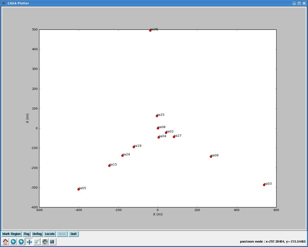
You'd like your reference antenna to be near the center of the array, and the easiest way to envision the array layout is with plotants.
#  plotants :: Plot the antenna distribution in the local reference frame:
vis                 = 'leotest.ms'      #  Name of input visibility file (MS)
figfile             =         ''        #  Save the plotted figure to this file
async               =      False        #  If true the taskname must be started using
                                        #   plotants(...)
will produce a plot that looks like this:
You can zoom and pan if you click on this icon: ![]() . Then, holding down your left mouse button and fiddling with the mouse will let you pan; holding down the right mouse button and fiddling with the mouse enables zooming in and out. Make note of an antenna near the center of the array, and check the observing logs to make sure nothing fishy happened to it during the observations. You can also take a quick look at the antenna in plotms to make sure it looks reasonably steady (we'll talk more about plotms below).
. Then, holding down your left mouse button and fiddling with the mouse will let you pan; holding down the right mouse button and fiddling with the mouse enables zooming in and out. Make note of an antenna near the center of the array, and check the observing logs to make sure nothing fishy happened to it during the observations. You can also take a quick look at the antenna in plotms to make sure it looks reasonably steady (we'll talk more about plotms below).
First Round of Data Flagging
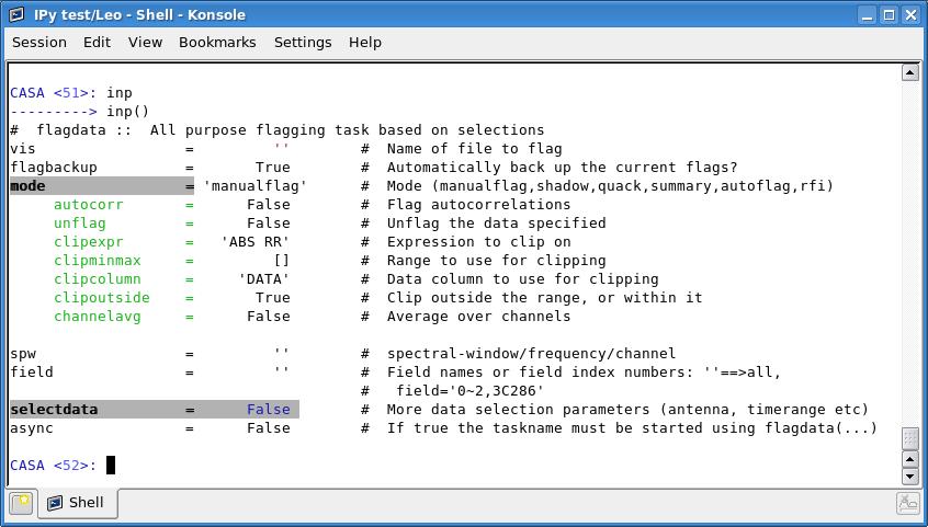
Oftentimes, the first few integrations of each scan are bad, and you'd like to flag them. This is called 'quack' a la AIPS, and is implemented using flagdata. This is what the default flagdata parameters look like in your CASA window:
Tip: You'll notice that some parameters are colored differently than others. Standard parameters (familiar from AIPS) are simple black text (like 'vis' above). Parameters which are shaded grey (like 'selectdata') are expandable, and once they have been expanded (like 'mode'), green sub-parameters (like 'autocorr') will appear. Note that if you were to change 'mode' from 'manualflag' to, say, 'quack', a different menu of green sub-parameters would appear.
To quack the first 10 seconds of each scan, set the flagdata parameters to:
#  flagdata ::  All purpose flagging task based on selections
vis                 = 'leotest.ms'      #  Name of file to flag
flagbackup          =       True        #  Automatically back up the current flags?
mode                =    'quack'        #  Mode (manualflag,shadow,quack,summary,autoflag,rfi)
     autocorr       =      False        #  Flag autocorrelations
     unflag         =      False        #  Unflag the data specified
     quackinterval  =         10        #  Quack n seconds from scan beginning/end
     quackmode      =      'beg'        #  Quack mode. 'beg' ==> beginning of scan. 'endb' ==> end of
                                        #   scan. 'end' ==> all but end of scan. 'tail' ==> all but
                                        #   beginning of scan
     quackincrement =      False        #  Flag incrementally in time?

spw                 =         ''        #  spectral-window/frequency/channel
field               =         ''        #  Field names or field index numbers: ''==>all,
                                        #   field='0~2,3C286'
selectdata          =      False        #  More data selection parameters (antenna, timerange etc)
async               =      False        #  If true the taskname must be started using flagdata(...)
Now is also the time to flag any obviously aberrant data in your calibrators. You might choose to flag with viewer, which displays a raster image of your uv data and is similar to SPFLG and TVFLG in AIPS (click here for an introduction to viewer). Alternatively, you can flag using a 2-dimensional interactive plot with plotms click here for an introduction to plotms). The plotting capabilities are similar to UVPLT in AIPS, and plotted points can be flagged (like WIPER in AIPS).

