Antennae Band7 - Imaging for CASA 3.3
Overview
This section of the AntennaeBand7 CASA Guide cover the imaging of the continuum and spectral line data. It begins where the Antennae Band7 - Calibration section left off. If you completed the Calibration section of the guide, then you may want to continue with the calibrated data sets. If you did not complete the Calibration section, then you can download the calibrated uv-data from the region closest to your location:
North America Europe East Asia
Then download the file 'Antennae_Band7_CalibratedData.tgz' to obtain the calibrated uvdata. Once the download has finished, unpack the file using 'tar -xvzf Antennae_Band7_CalibratedData.tgz' and change directory (cd) to Antennae_Band7_CalibratedData. You should have Antennae_South.ms and Antennae_North.ms in your working directory. Then start CASA with the 'casapy' command.
Continuum Imaging
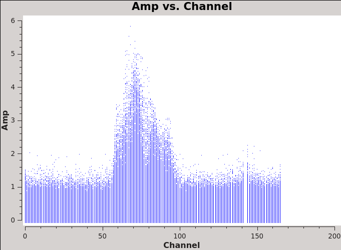
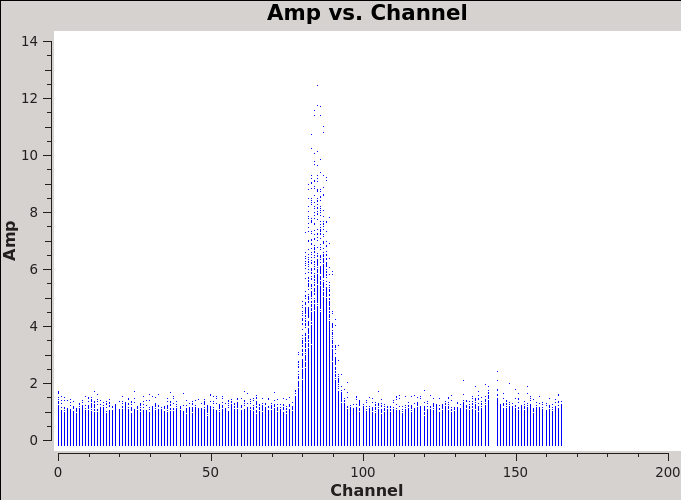
We will make 345 GHz continuum images for the two regions covered by the mosaics. We use the task clean over the channels that are free of the line emission; we avoid the edge channels which tend to be noisier due to bandpass rolloff effects. The line-free channels are found by plotting the average spectrum. We find the CO(3-2) line from channels 50 to 100 in the southern mosaic, and from 70 to 100 in the northern mosaic.
# In CASA
plotms(vis='Antennae_South.cal.ms',xaxis='channel',yaxis='amp',
      avgtime='1e8',avgscan=T)
plotms(vis='Antennae_North.cal.ms',xaxis='channel',yaxis='amp',
      avgtime='1e8',avgscan=T)
The *avgtime* is set to a large value so that it averages over all the integrations, and *avgscan* is set to allow averaging of the different scans.
Next we create continuum images from the line-free channels.
Northern Continuum Mosaic
For illustrative purposes we first make a dirty image to see if there is emission and what the exact beam size is. It should be on the order of 1" but this will vary a bit according to the uv-coverage in the actual data. We will start with a cellsize of 0.2" to oversample the beam by a factor of 5. The imsize needs to be large enough given the cell size to comfortably encompass the mosaic. From the mosaic footprints shown at AntennaeBand7#ALMA_Data_Overview we can see that Northern mosaic size needs to be about 1 arcmin. At 2" this requires a imsize=300
# In CASA
os.system('rm -rf Antennae_North.Cont.Dirty*')
clean(vis='Antennae_North.cal.ms',imagename='Antennae_North.Cont.Dirty',
     field='',phasecenter='12',
     mode='mfs',restfreq='345.79599GHz',
     spw='0:1~50;120~164',
     imagermode='mosaic',
     imsize=300,cell='0.2arcsec',
     interactive=F,
     niter=0, threshold='0.5mJy')
The reported beam size is 1.26" x 0.66" P.A. 86.045 degrees.
NOTE:clean will generate several files automatically with the imagename prepended:
- <imagename>.image # the final restored image
- <imagename>.flux # the effective primary beam response (e.g. for pbcor)
- <imagename>.flux.pbcoverage # the primary beam coverage (ftmachine=’mosaic’ only)
- <imagename>.model # the model image
- <imagename>.residual # the residual image
- <imagename>.psf # the synthesized (dirty) beam
# In CASA
viewer('Antennae_North.Cont.Dirty.image')
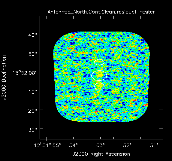
Yes there is definitely a detection in the vicinity of the Northern nucleus (see Fig. 4 below). Using the square region icon, and drawing a box near but not including the emission, we find the rms noise is about 0.4 mJy/beam in the dirty image.
Next we switch to refined values of cell=0.13" and imsize=500 based on the observed beam size. We also switch to interactive mode so that you can create a clean mask using the polygon tool (note you need to double click inside the polygon region to activate the mask. See TWHydraBand7_Imaging#Image_and_Self-Calibrate_the_Continuum for a more complete description of clean mask creation.
Note that if you run the clean task again with the same *imagename*, without deleting the existing <imagename>.* files, clean assumes that you want to continue cleaning the existing images.
# In CASA
os.system('rm -rf Antennae_North.Cont.Clean*')
clean(vis='Antennae_North.cal.ms',imagename='Antennae_North.Cont.Clean',
     field='',phasecenter='12',
     mode='mfs',restfreq='345.79599GHz',
     spw='0:1~50;120~164',
     imagermode='mosaic',
     imsize=500,cell='0.13arcsec',
     interactive=T,
     niter=1000, threshold='0.5mJy')
The input parameters include:
- vis='Antennae_North.cal.ms': The calibrated dataset on the science target
- imagename='Antennae_North.Cont.Clean': The base name of the output images
- phasecenter='12': the source id of the mosaic.
- spw='0:0~50,0:120~164': To specify only the line-free channels of spectral window 0.
- mode='mfs': Multi-Frequency Synthesis: The default mode, which produces one image from all the specified data combined
- niter=1000: Maximum number of clean iterations -- *we will stop interactively*
- theshold='0.5mJy': Stop cleaning if the maximum residual is below this value (the dirty rms noise)
- imsize=500, cell='0.2arcsec': Image size in pixels, chosen to cover the mosaic, and the cell size per pixel in arcsec to properly sample the synthesized beam (at least three times).
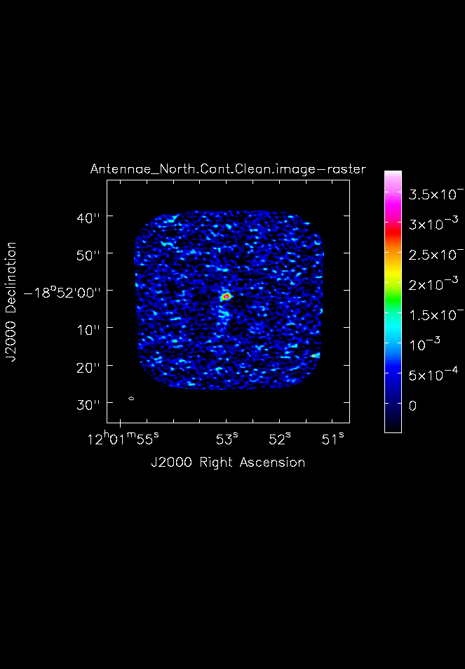
Southern Continuum Mosaic
For the southern mosaic we modify the phase center and the line-free channels:
# In CASA
os.system('rm -rf Antennae_South.Cont.Clean*')

clean(vis='Antennae_South.cal.ms',imagename='Antennae_South.Cont.Clean',
     field='',phasecenter='15',
     mode='mfs',restfreq='345.79599GHz',
     spw='0:0~30,0:120~164',
     imagermode='mosaic',
     imsize=700,cell='0.13arcsec',
     interactive=F,
     niter=1000, threshold='0.5mJy')
The Half Power Beam Width (HPBW) of the elliptical synthesized beam is:
- Northern mosaic: 1.28" times 0.66", with a position angle (PA) equal to 86 deg.
- Southern mosaic: 1.15" times 0.66", and PA equal to 68 deg.
We will determine some statistics for the images using the task imstat:
# In CASA
imstat('Antennae_North.Cont.Clean.image')
imstat('Antennae_South.Cont.Clean.image')
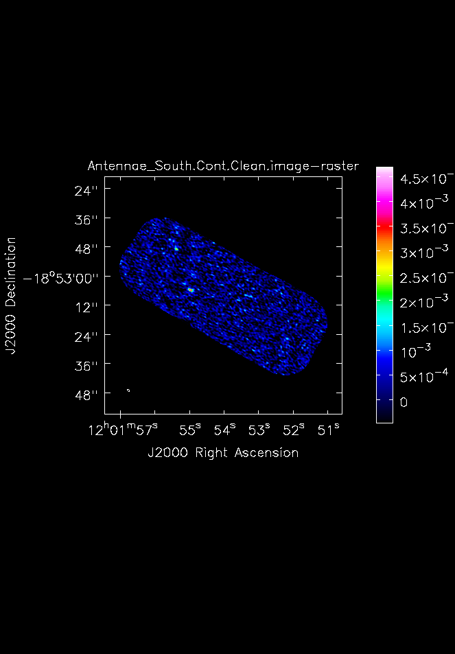
The peak flux densities of the images are ~4.4 and 2.9 mJy for the southern and northern mosaics, and both have a similar rms ~ 0.3 mJy, thus the obtained dynamic ranges are larger or equal than 10.
Now we will plot the results using imview to obtain Figures 4 and 5:
# In CASA
imview (
  raster={'file': 'Antennae_North.Cont.Clean.image',
  'colorwedge':T,},
  zoom=1, out='Antennae_North.Cont.Clean.image.png')
imview (
  raster={'file': 'Antennae_South.Cont.Clean.image',
  'colorwedge':T,},
  zoom=1, out='Antennae_South.Cont.Clean.image.png')
CO(3-2) Imaging
Continuum subtraction
Such continuum emission is too small to have any significant effect on the line. However, it is educative to subtract the continuum emission in the uv-domain using the task uvcontsub.
# In CASA

uvcontsub(vis = 'Antennae_North.cal.ms',
	  fitspw='0:5~50,0:120~164', solint ='inf',
	  fitorder = 1, fitmode = 'subtract')

uvcontsub(vis = 'Antennae_South.cal.ms',
	  fitspw='0:5~30,0:120~164', solint ='inf',
	  fitorder = 1, fitmode = 'subtract')
where:
- fitspw='0:5~50,0:120~164': Correspond to the line-free channels
- fitorder = 1: We substract just a first-order polynomial
- fitmode = 'subtract': Subtract the continuum from all channels. Note that the result is stored in the CORRECTED_DATA column
Clean CO(3-2) line
Next, we clean the CO(3-2) line emission with the following instances:
# In CASA
os.system('rm -rf Antennae_North.Line*')
clean(vis='Antennae_North.cal.ms',
     imagename='Antennae_North.Line.Clean',
     spw='0',field='',phasecenter='12',
     mode='velocity',outframe='LSRK',restfreq='345.79599GHz',
     nchan=60,start='1300km/s',width='10km/s',
     imagermode='mosaic',
     imsize=500,cell='0.13arcsec',minpb=0.2,
     interactive=T,
     weighting='briggs',robust=0.5,
     niter=10000, threshold='5.0mJy')

os.system('rm -rf Antennae_South.Line*')
clean(vis='Antennae_South.cal.ms',
     imagename='Antennae_South.Line.Clean',
     spw='0',field='',phasecenter='15',
     mode='velocity',outframe='LSRK',restfreq='345.79599GHz',
     nchan=60,start='1300km/s',width='10km/s',
     imagermode='mosaic',
     imsize=1000,cell='0.13arcsec',minpb=0.2,
     interactive=T,
     weighting='briggs',robust=0.5,
     niter=10000, threshold='5.0mJy')
Note that you can obtain the dirty maps first by setting niter=0.
Notable parameters include:
- mode='velocity',outframe='LSRK',restfreq='345.79599GHz'. We use 'velocity' mode to set velocity information in the Local Standard of Rest frame, and use the rest frequency of the CO(3-2) line.
- nchan=60,start='1300km/s',width='10km/s': To produce a data cube with 60 channels("nchan"=60), starting at 1300km/s and with velocity widths of 10 km/s. That will include all the CO(3-2) emission in both mosaics.
- imsize=1000,cell='0.13arcsec'. An image size of 130 arcsec, with pixels of 0.13 arcsec (~ 5 times the minor axis of the synthesized beam). We make the imsize larger than the mosaic to increase the dirty beam image size, as the emission is quite extended along the mosaic.
- weighting='briggs',robust=0.5: Weighting to apply to visibilities. We use Brigg's weighting and robustness parameter 0.5 (in between natural and uniform weighting).
- niter=10000: Maximum number of clean iterations.
- threshold='5.0mJy': Stop cleaning if the maximum residual is below this value.
The threshold is ~ 2 the rms of the line-free channel for each dataset.
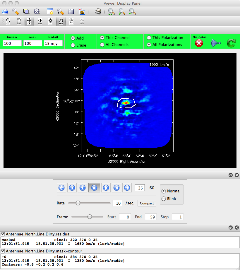
Using interactive=T the viewer will open when it is ready to start an interactive clean. Step through to the channels to see how extended the emission is and choose a region for each channel. You can also choose "All Channels" if you want to define the same clean mask for all channels. Note that when you define a polygon region, it is needed to double click inside it to save the mask region. You can select as many regions as you need. You can use the "tape deck" to step through the channels again and check that the emission in all channels fits within the mask(s) you have created. See an example of selected region for a given channel in Figure 5. To continue with clean use the "Next action" button in the green area on the Viewer Display GUI: The red X will stop clean where you are; the blue arrow will stop the interactive part of clean, but continue to clean non-interactively until reaching the stopping niter or threshold (whichever comes first); and the green arrow will clean until it reaches the "iterations" parameter on the left side of the green area.
When the cleaning has finished, you may want to inspect the resulting data cubes:
imview (raster={'file': 'Antennae_North.Line.Clean.image'})
imview (raster={'file': 'Antennae_South.Line.Clean.image'})
The (line-free) channel rms for the northern and southern mosaics are 2.7 mJy/beam and 2.4 mJy/beam, respectively, for 2.3 and 3.8 hours times on source approximately. The ALMA sensitivity calculator gives an on-source observing time of ~3-4 hours to reach a noise level of 2.5 mJy using 12 antennas for an angular resolution of 1 arcsec. Note that the fields are overlapping by 0.5 the size of the primary beam. Note however that the dynamic range is worse than that. Self-calibration and multiscale will help improving this situation.
Self calibration and multi scale cleaning
We will update this section soon.
Moment maps
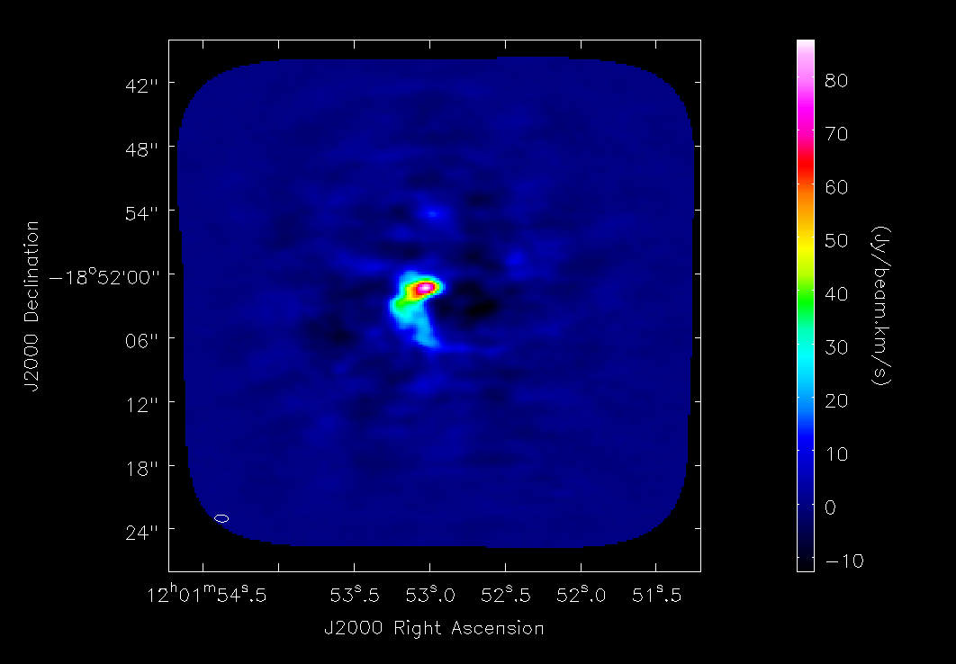
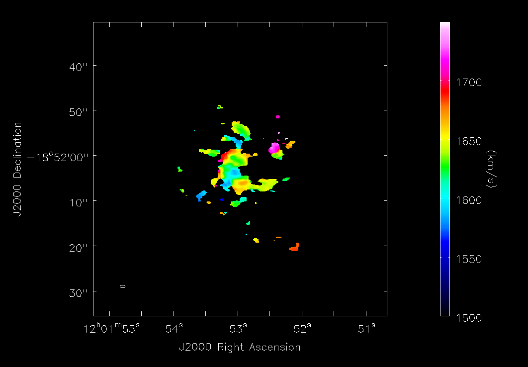
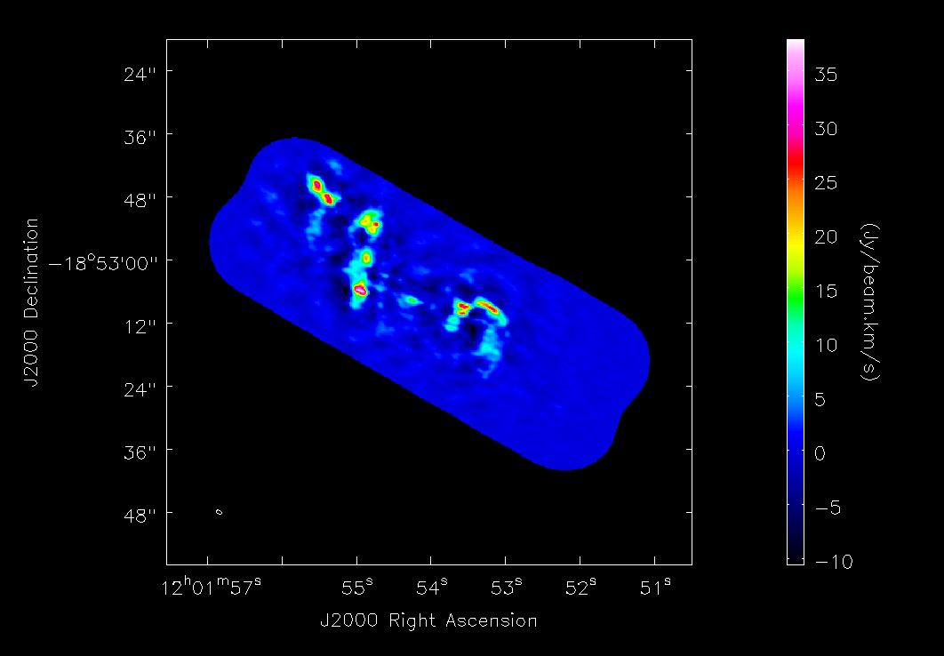
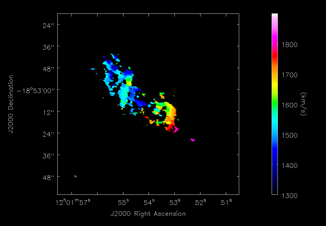
Next, we make the integrated intensity maps and velocity fields of the CO(3-2) emission using the task immoments. Note that we choose to run the immoments separately for the total intensity map and the velocity field because we want to use different flux thresholds.
For the northern mosaic the moment 0 and 1 can be calculated as follows:
# In CASA
os.system('rm -rf Antennae_North.Line.Clean.Mom.image*')
immoments('Antennae_North.Line.Clean.image',
   moments=[0], axis="spec",
 outfile='Antennae_North.Line.Clean.Mom.image.integrated')

os.system('rm -rf Antennae_North.Line.Clean.Mom.Mask.image.weighted_coord*')
immoments('Antennae_North.Line.Clean.image',
   moments=[1], axis="spec",
    mask="Antennae_North.Line.Clean.image>4.e-2",
   outfile='Antennae_North.Line.Clean.Mom.Mask.image.weighted_coord')
And for the southern mosaic:
# In CASA
os.system('rm -rf Antennae_South.Line.Clean.Mom.image*')

immoments('Antennae_South.Line.Clean.image',
   moments=[0], axis="spec",
   outfile='Antennae_South.Line.Clean.Mom.image.integrated')

immoments('Antennae_South.Line.Clean.image',
   moments=[1], axis="spec",
   mask="Antennae_South.Line.Clean.image>2.5e-2",
   outfile='Antennae_South.Line.Clean.Mom.Mask.image.weighted_coord')
where:
- moments=[x]: To specify that we wish to make the xth moment map. The 0th moment map gives integrated emission and the 1st gives the intensity-weighted velocity field
- axis='spectral': Indicates the moment axis; in this case, 'spectral'
- mask="Antennae_North.Line.Clean.image>X" Mask applied to the image before calculating the moments. Consider pixels in Antennae_North.Line.Clean.image that are larger than X
- outfile='Antennae_South.Line.Clean.Mom.image.XX': The output image name
Finally, we visualize the different moments using imview:
# In CASA
imview (
  raster={'file': 'Antennae_North.Line.Clean.Mom.image.integrated',
  'colorwedge':T,},
  zoom=1, out='Antennae_North.Line.Clean.Mom.image.integrated.png')

imview (
   raster={'file': 'Antennae_North.Line.Clean.Mom.Mask.image.weighted_coord',
   'range': [1500,1750],'colorwedge':T},
   zoom=1, out='Antennae_North.Line.Clean.Mom.Mask.image.velfield.png')

imview (
   raster={'file': 'Antennae_South.Line.Clean.Mom.image.integrated',
   'colorwedge':T},
   zoom=1,out='Antennae_South.Line.Clean.Mom.image.integrated.png')

imview (
   raster={'file': 'Antennae_South.Line.Clean.Mom.Mask.image.weighted_coord',
   'range': [1300,1900],'colorwedge':T},
   zoom=1, out='Antennae_South.Line.Clean.Mom.Mask.image.velfield.png')
Comparison with previous SMA CO(3-2) data
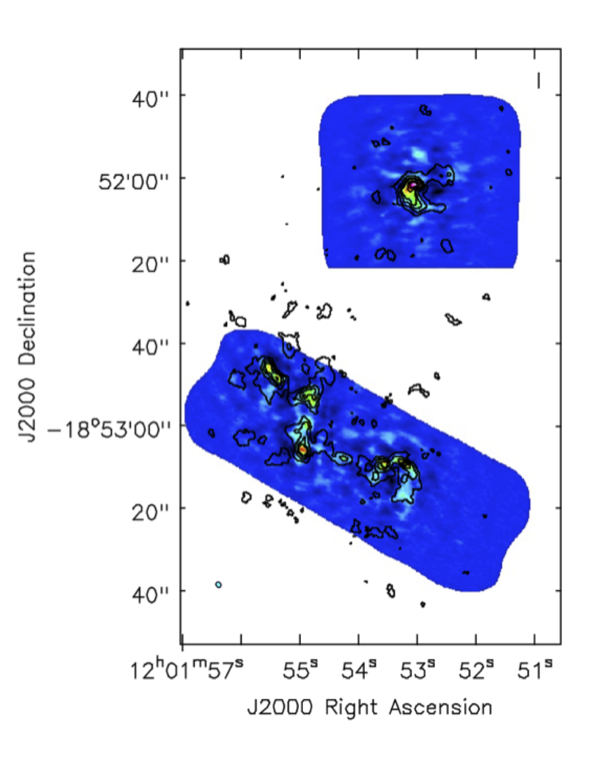
We compare with SMA CO(3-2) data (Ueda, Iono, Petitpas et al., in preparation, to be submitted to ApJ). Figure 13 shows a comparison plot betwee the moment 0 maps of ALMA and SMA data using the viewer. The fluxes, peak locations and large scale structure are consistent. Both southern and northern components have been combined.
Exporting to Fits
You can convert from CASA format to FITS if you want to analyze the data using another software package. If you have difficulty with the standard FITS output from CASA, try setting velocity=T and/or dropstokes=T.
# In CASA
exportfits(imagename='Antennae_North.Line.Clean.image',
     fitsimage='Antennae_North.Line.Clean.image.fits')
exportfits(imagename='Antennae_North.Line.Clean.Mom.image.integrated',
     fitsimage='Antennae_North.Line.Clean.Mom.image.integrated.fits')
exportfits(imagename='Antennae_North.Line.Clean.Mom.Mask.image.weighted_coord',
     fitsimage='Antennae_North.Line.Clean.Mom.Mask.image.weighted_coord.fits')
# In CASA
exportfits(imagename='Antennae_South.Line.Clean.image',
     fitsimage='Antennae_South.Line.Clean.image.fits')
exportfits(imagename='Antennae_South.Line.Clean.Mom.image.integrated',
     fitsimage='Antennae_South.Line.Clean.Mom.image.integrated.fits')
exportfits(imagename='Antennae_South.Line.Clean.Mom.Mask.image.weighted_coord',
     fitsimage='Antennae_South.Line.Clean.Mom.Mask.image.weighted_coord.fits')
Daniel Espada 12:00 UT, 27 July 2011