Calibrating a Mosaicked Spectral Line Dataset
This tutorial assumes you have extracted your data from native MIRIAD format to FITS files for each spw (see Extracting data from MIRIAD).
Note: This tutorial details a particular calibration path optimized for the example dataset being used; in cases where alternative command calls are described, these commands are commented out. This formatting allows them to be extracted with all other CASA commands in this tutorial by the automated script extractor, and you can uncomment them if you wish to try them. See Extracting scripts from these tutorials for more information.
Importing your data into a CASA MS
Before looking at the data itself, we need to import the MIRIAD FITS files and use them to construct a CASA measurement set (MS). This tutorial assumes the FITS files are in a subdirectory called 'fits'. It also assumes that you have put the filename of the MS to be made into a global CASA variable, which is the same root as the output FITS files. The following variables could be defined either on the command line inside CASA, or in an executable python script:
# In CASA
fitsdir='fits/'
msdir='./'
project='c0104I'
msfile=msdir+project+'.ms'
Here are two possible ways to import your FITS files into CASA; one relies more on CASA structures, and the other on basic python syntax (this second one is currently commented out). You only need to run one, but see which one makes more sense to you.
Method 1
This method creates a python dictionary and uses "for" loops in python to run importuvfits multiple times, and then uses the output as the input to the concat task.
myfiles = []
for i in range(4,7):
        msfile = project+str(i)+'.ms'
        importuvfits(fitsfile=fitsdir+project+str(i)+'.fits',
                     vis=msfile)
        myfiles.append(msfile)
concat(vis=myfiles,concatvis='c0104I',timesort=True)
Method 2
This method uses some basic python utilities. You can use the following "for" loop to read each of the individual FITS files directly into an MS of the same name (e.g., for a FITS file named "c0104I.4.fits", produce an MS called "c0104I.4.ms" .) The following lines then concatenate the individual spectral windows MS directories into one big MS containing all spectral windows, for all sources, using concat.
# in CASA
#from glob import glob as filesearch
#import os
#
#inlist = sorted(filesearch(fitsdir+'*.fits'))
#for item in inlist:
#    infile=item.split('/')[-1]
#    outfile=infile.replace('.fits','.ms')
#    importuvfits(fitsfile=item, vis=msdir+outfile)
#files = sorted(filesearch('*.ms'))
#concat(vis=files,concatvis=catfile,freqtol="",dirtol="1arcsec",async=False)
Now you can proceed with examining and calibrating the data.
Examining your data
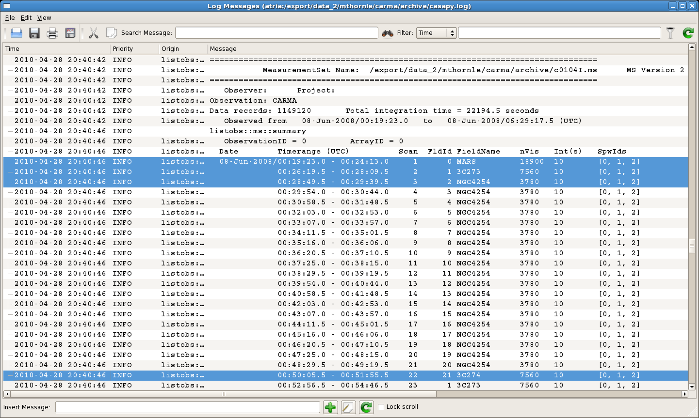
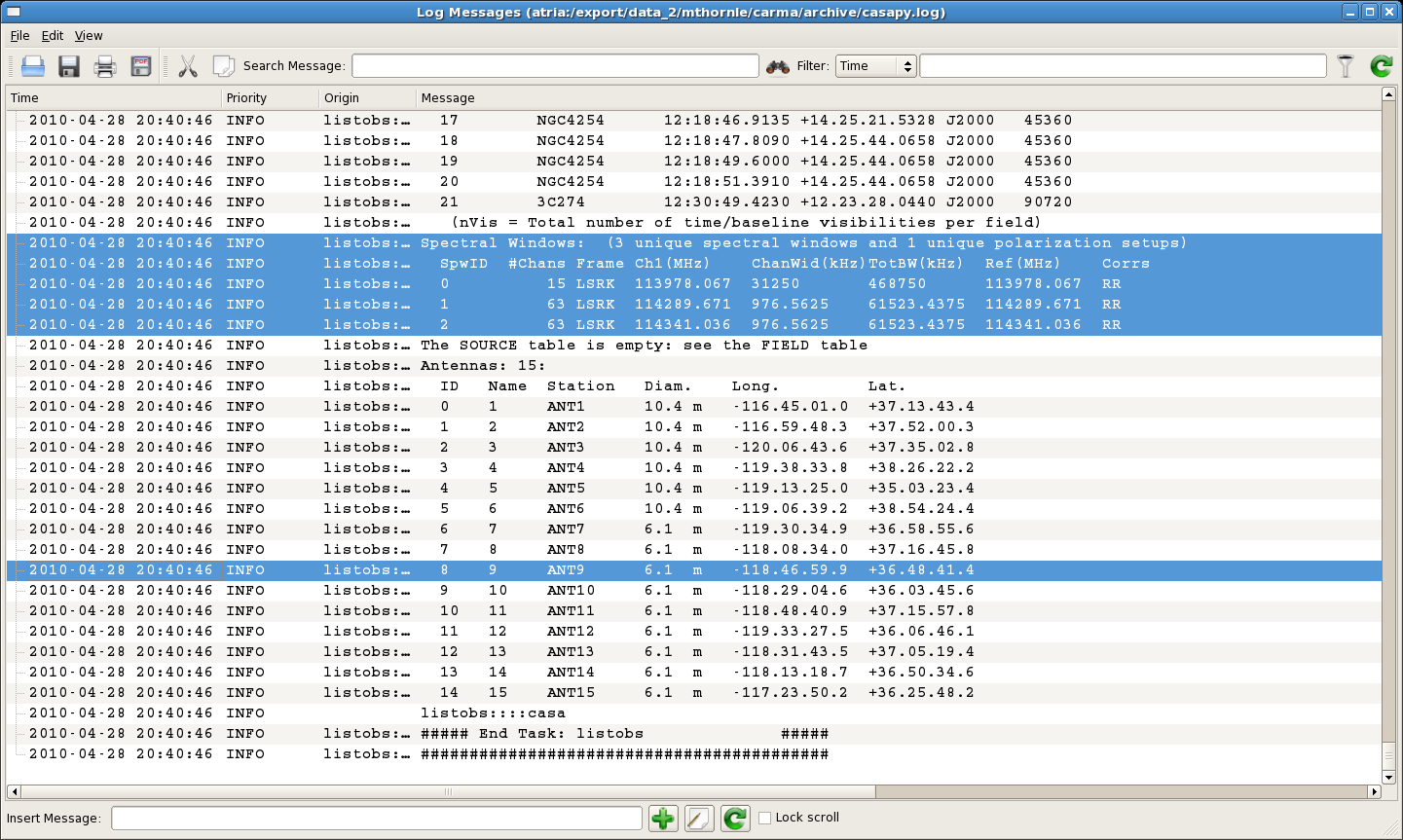
You'll need some information about the IDs that CASA assigns to your calibrators, sources, and antennas. So if you haven't yet done so,
# In CASA
listobs(vis=msfile)
You will want to look through the listobs output to determine:
- The Field ID (FldId) or source name (as listed in the header) of each of your sources and calibrators.
- The Spectral Window ID (SpwID) of each spectral window you want to calibrate.
- The Name (or station; the ID number is actually least useful) of your reference antenna.
Near the beginning of the listobs output, you will find the first listing of FldId numbers. Any "field=" input can be filled with either the object's Field ID or source name. In this example, the flux calibrator (MARS) is assigned FldId=0, the bandpass (and phase) calibrator (3C273) is assigned FldId=1, the mosaicked source fields are assigned FldId 2 through 20 (that's field='2~20' in python), and an extra "test" calibrator was also observed (3C274) and assigned FldId=21. CASA does not yet have full functionality for using planets as calibrators (it's expected for the next release), so for this tutorial we will use 3C273 as flux, bandpass, and phase calibrator.
Near the end of the listobs output, you will find listings of the properties of the observed spectral windows, and the locations of the antennas. In this case, the narrowband windows are assigned to SpwID of 1 and 2, and they each have 63 channels. The reference antenna is Antenna 9, which unfortunately here is named '9'. For unambiguous antenna selection, ideally the Name (which CASA searches first) should have text in it; if it does not, you may want to use the unambiguous Station name of 'ANT9' to ensure that CASA chooses the right antenna.
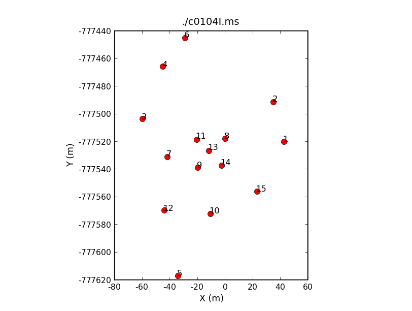
If you'd prefer a graphical representation of antenna positions in order to choose your reference antenna, you can use plotants. The following command
# In CASA
plotants(vis=msfile,figfile='plotants.png')
will display the physical layout of the antennas.You can see antenna 9 near the middle of the CARMA antenna distribution.
Beta-alert: At the time of this revision (CASA 3.2), plotants was leaving table.lock files that make the rest of the tutorial unhappy. Here's a pythonic way to zap those table.lock files.
import os
for root, dirs, files in os.walk('./'):
    for name in files:
        if name == 'table.lock': os.remove(os.path.join(root,name))
Doing a little flagging
Before proceeding with your calibration, it is a good idea to flag any obviously bad data up front. See Data flagging with plotms or Data flagging with viewer for more detailed instructions on looking for bad data and on flagging interactively; as a practical counterpoint, we provide here some straightforward examples of non-interactive flagging.
You can examine your visibility data by typing
# In CASA
plotms(vis=msfile)
In plotms you can examine the data for different sources, antennas, time ranges, spw, etc. by entering your selections in the 'Data' tab that is open when you start plotms. For the data used in these tutorials, the data generally look quite clean, but there are some noisy data. Here we give instructions for flagging these data non-interactively, including commands for other typical flagging: data from shadowed antennas, and the end channels of each spw.
Use flagdata to tell CASA which data you want flagged. The first two flagging commands indicate how to flag shadowed data, and how to flag two channels on each end of each spw. (Remember, for these data there is one wideband spw with 15 channels and two narrowband spw with 63 channels each. Also remember that CASA and python start counting at 0, not 1.)
# In CASA
flagdata(vis=msfile,mode='shadow',diameter=-1)
flagdata(vis=msfile,mode='manualflag',selectdata=True,spw='0:0~1;13~14')
flagdata(vis=msfile,mode='manualflag',selectdata=True,spw='1~2:0~1;61~62')
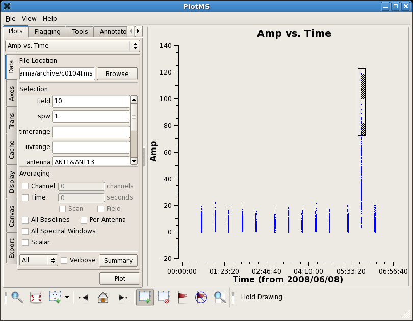
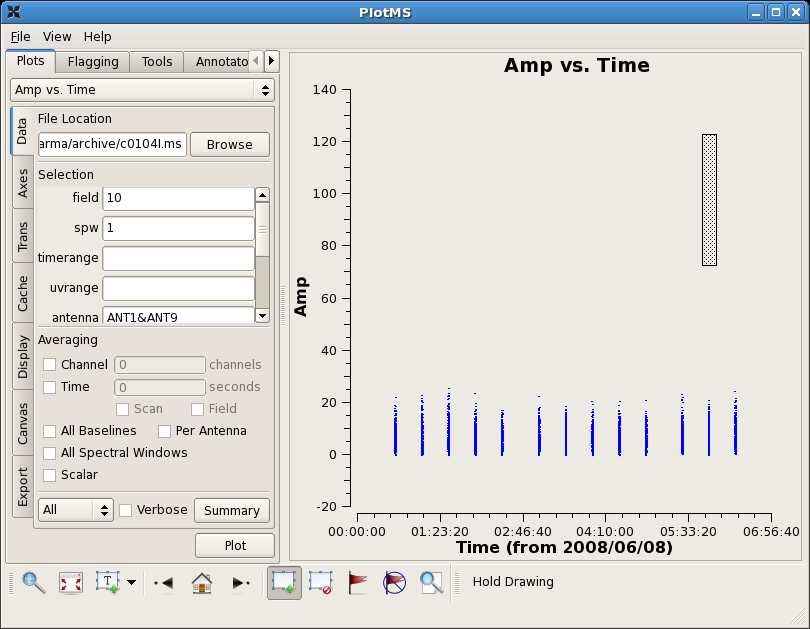
Next we will look for noisy data. The flagdata command allows for quite complex flagging, so let's first start with a relatively straightforward example: we will flag this one noisy time range, for the offending antenna and for all the fields in which high amplitudes are seen. The station name is used for 'antenna=' to make it unambiguous, and individual field numbers are specified here, because only a subset of on-source fields actually show noisy data. You can use zoom, mark, and locate, using the icons at the bottom of the plotms GUI to look for a pattern.
# In CASA
flagdata(vis=msfile,mode='manualflag',selectdata=True,spw='0~2',
         antenna='ANT13',field='2~11',timerange='05:41:00~05:55:00')
With more investigation, you can see using plotms that the first two scans on 3c273 and the last scan on 3c273 show some low points. Again use zoom, mark, and locate to see if you can see a pattern.
The first two scans on 3c273 don't show a particular pattern; no particular antenna or individual time range appears to be responsible. This is usually a good indication that it cannot be calibrated out. Also note that it is unlikely that the target data in between is good, though this is not obvious because the target is weak. However, 3c274 does look ok, before the second 3c273 scan. Unfortunately, there is no way to calibrate the first scans on the source even if they are good, with no calibrator scan to precede them. For now we will flag scans on 3c273 and the source in that timerange.
As for the last scan, there is a pattern: problems with the last scan on 3c273 appears to be caused by antenna ANT7 (in scan 272) and problems with the last scan on 3c274 appears to be related to antenna ANT8 (scan 255).
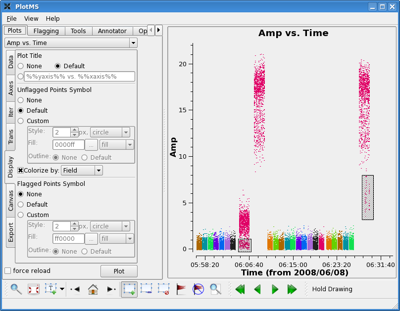
Looking at the lowest points on all the 3c273 scans, baseline ANT2-ANT8 appears low, we will also wait to see if this calibrates out.
We will flag the narrow band channels wherever we see problems in wideband. You can either make separate plotting commands, or combine as below, which flags all of the suspect data we have described here. To demonstrate different possibilities we use timerange to identify some data, and scan number others. To understand what will be flagged, put together the same element of each of the antenna,field,scan, and timerange arrays. You can see, for instance, the first element of each of these arrays describes the flagging that was done in the simpler flagging command above.
flagdata(vis=msfile,spw='0~2',
	 antenna=['ANT13','','ANT7','ANT8'],
	 field=['2~11','1~20','1','21'],
	 scan=['','','272','255'],
	 timerange=['05:43:00~05:54:00','00:25:00~00:55:00','',''])
Note that each of these flagging commands could have been written out separately, but combining them into one command will run much faster than the combined time of multiple calls as the data only have to be searched once.
Calibrating your data
Before running your calibration, it's a good idea to run the following command:
# In CASA
clearcal(vis=msfile)
If this is the first time you've calibrated, clearcal won't do much, but it will initialize table columns that might be missing from the import step (you may see some output to the log screen to this effect). If you are trying a new calibration, this command ensures your data returns to their original state. So it can't hurt you, and can help.
Calibration in CASA consists of creating calibration tables, and then applying them as needed. Here, we step you through bandpass, gain, and amplitude calibration, and then indicate how to apply them to your source data.
Bandpass calibration
The following command (bandpass) will create a bandpass calibration table (caltable=) using the specified bandpass calibrator (field=) and reference antenna (refant=), and places it in the same directory as the data are found. For these data, 3C273 is a good bandpass calibrator, but as it is also used as a phase calibrator (and therefore observed over several hours) an intial phase-only gain calibration is needed to take out phase drifts. Only the central subset of channels in each spw is used, since the bandpass correction has not yet been applied.
# In CASA
gaincal(vis=msfile,caltable=msdir+project+'.initphasecal',
        field='3C273', spw='0:3~10,1~2:20~40',calmode='p',
        gaintype='G',minsnr=2.0, refant='ANT9', solint='inf', combine='')
Now provide this phase-only gaincal table to bandpass, by putting the table name into gaintable= and the calibrator name into gainfield= (in this case, 3C273 is the only field in the gaincal table, so you could also leave gainfield unspecified.)
# In CASA
default('bandpass')
bandpass(vis=msfile,caltable=msdir+project+'.bcal',gaintable=msdir+project+'.initphasecal',gainfield='3C273',
         interp='',field='3C273',spw='',bandtype='B',solint='inf',refant='ANT9',
         solnorm=True)
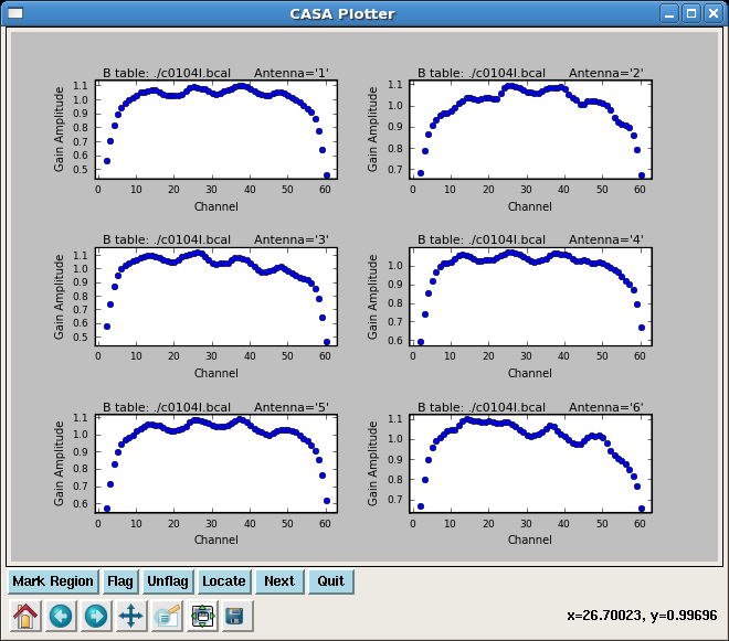
You can look at the bandpass calibration table you've created using plotcal. This first call will plot the *.bcal table to a GUI for you to look at and interact with--here, you are looking at one of the narrowband spectral windows (spw='1'), and making a 3x2 display of bandpass plots, one for each antenna:
# In CASA
plotcal(caltable=msdir+project+'.bcal',xaxis='chan',yaxis='amp',
        iteration='antenna',subplot=321,spw='1',
        showgui=T)
This second call outputs the same kind of plot to a PNG file (filename specified by 'figfile') without opening the interactive GUI:
# In CASA
plotcal(caltable=msdir+project+'.bcal',xaxis='chan',yaxis='amp',
        iteration='antenna',subplot=321,spw='1',
        showgui=F,figfile='bp_spw1')
Amplitude and gain calibration
3C273 was used as a phase calibrator for this observation, but it is strong enough to serve as bandpass and flux calibrator as well, so we will use it for all aspects of calibration in this example. As in AIPS the task setjy is used to provide source information for objects of known flux and distribution. You can use the CARMA flux calibrator database to determine the flux of your flux calibrator at the time of your observation. For these observations, the flux of 3C273 was recorded as 17.8 Jy. You can provide this information to CASA using the following command:
# In CASA
setjy(vis=msfile, field='3C273',fluxdensity=[17.8,0.,0.,0.], spw='0~2')
The task gaincal can then be used to determine the appropriate gains to be applied as a function of time. 3C273 is a nice strong calibrator, so we can determine the gain calibration with time for each spw individually. (If there is no amplitude or phase offset between the wide and narrow spw's, you could also use the wideband spw and apply it to each narrowband spw; this may be valuable in the case of a weaker calibrator.) As before, and we have used the station title of the reference antenna (refant='ANT9') to unambiguously identify it.
The bandpass calibration table, specified here by gaintable, is accounted for prior to determining the gain table, so that the two calibrations remain separate. Note: neither the gain or bandpass calibration is actually applied to the source data here; both calibrations will need to be applied after they have been determined, using applycal (see below).
# In CASA
gaincal(vis=msfile,caltable=msdir+project+'.gcal',gaintable=msdir+project+'.bcal',
        gainfield='3C273', field='3C273', spw='',
        gaintype='G',minsnr=2.0, refant='ANT9', solint='inf', combine='')
Note: To use only the wideband spw for all gain calibration, you would set spw='0' for this dataset. To include another calibrator in your gain solutions, include its name or Field ID in the 'field' parameter, e.g., field='3c273,3C274' .
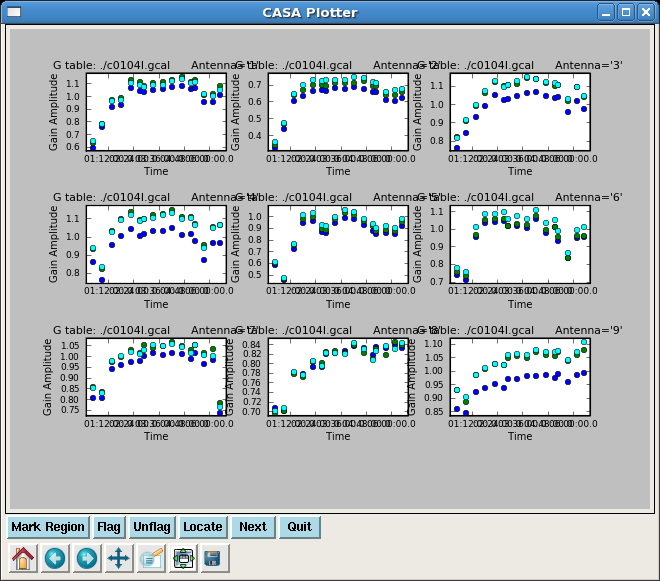
As before with the bandpass calibration table, you can see what the gain calibration table looks like with plotcal (in this example, using the phase calibrator 3C273):
# In CASA
plotcal(caltable=msdir+project+'.gcal', yaxis='amp',field='3C273',
        iteration='antenna',subplot=331,
        showgui=T)
Now that the gains have been determined, you can bootstrap the flux of 3C273 to any other calibrators, using fluxscale. This command uses the gain table (specified by caltable) and needs to be told which source has a known flux (reference=). In this example, we are also using 3C273 as the phase calibrator, so fluxscale is not needed, but if we wanted to use 3C274 as a calibrator as well we would need to transfer fluxes over using fluxscale. (Note: if there are no other calibrators in your gain calibration, CASA will complain and this call to fluxscale will likely cause your script to stop. Make sure to include these calibrators in your call to gaincal.)
# In CASA
# uncomment if your phase calibrator is distinct from your flux calibrator
#fluxscale(vis=msfile,caltable=msdir+project+'.gcal',
#          fluxtable=msdir+project+'.fcal', reference='3C273')
Note: All of the information from the gain table is contained in the flux table, so in the end, you will apply the bandpass and flux calibration tables in order to apply all relevant calibrations to your source data.
Applying your calibrations
Now that you have solutions for both bandpass and gain calibration, you can apply them to your data. Note that applycal does not operate on the raw data in this step, so you do not need to create a copy of the data before proceeding. Use of the command clearcal will return your data to a pristine state, if needed.
The task applycal is fairly flexible, allowing you to apply multiple calibration tables, and calibrations from one spectral window to others (however, you may need to consider the task accum if you have multiple pairs of sources and calibrators in the same dataset; see section 4.3 ('Apply the calibrations') of Calibrating a VLA 5 GHz continuum survey for an example using VLA data).
Here are two examples of applying calibrations, but these are still relatively simple. Consult the helpfile for applycal for a detailed explanation of how to use this command--note in particular the use of the parameter spwmap.
In the first example, we apply calibrations to the bandpass/flux/phase calibrator (field='3C273', or field='1'). We apply both bandpass and flux calibration tables. The order of entries in gainfield and spwmap are the same as for gaintable: in this case, it means that we take the bandpass calibration for 3C273 (gainfield=['3C273',...) and apply the solutions for each spectral window to the same spectral window for the other sources (spwmap=[[],...), and we do the same for the gain/flux calibration (gainfield=...,'3C273'],spwmap-...,[]]). If you had determined the gain/flux calibration using the wideband channel only (spw='0'), you would apply that calibration to all spectral windows by fixing the second term of spwmap (spwmap=...,[0]]).
You would only need to do this first example if you wanted to image the bandpass/flux/phase calibrator 3C273.
# In CASA
# uncomment to apply 3C273 calibrations to itself, if you want to image 3C273
#applycal(vis=msfile,field='3C273',spw='',
#         gaintable=[msdir+project+'.bcal',msdir+project+'.gcal'],
#         gainfield=['3C273','3C273'],spwmap=[[],[0]])
In this second example, we apply bandpass and flux calibrations to the source (or any other object in the dataset you want to image). In this case, we use the gain/flux calibration information for 3C273 to apply to the source. Note:If you run the fluxscale command above because you are using separate sources for flux and gain calibration, replace the '.gcal' above with'.fcal'.
# In CASA
applycal(vis=msfile,field='2~20',spw='',
         gaintable=[msdir+project+'.bcal',msdir+project+'.gcal'],
         gainfield=['3C273','3C273'],spwmap=[[],[]])
Calibration is now complete! Proceed onward to Imaging a Mosaicked Spectral Line Dataset.
↵ CARMA Tutorials
↵ CASAguides
Last checked on CASA Version 3.0.1 (r10803).