VLA Self-calibration Tutorial-CASA6.4.1
This CASA Guide is for Version 6.4.1 of CASA, and was last checked with CASA 6.5.4.
Introduction
After calibrating a data set using the observed calibrator sources (standard calibration), there may be residual phase and/or amplitude errors in the calibrated data of the target source that degrade the image quality. Self-calibration (selfcal) is the process of using a model of the target source to reduce the phase and amplitude errors in the visibilities of the same target source. While some other CASA guides include a self-calibration step, this guide describes the process in greater detail, including how to optimize parameters to achieve the best result.
Fundamentally, self-calibration is almost identical to standard calibration. Both standard calibration and selfcal work by comparing the visibility data with a model to solve for calibration solutions. With standard calibration, we are usually provided a model of our calibrator source by the observatory (e.g., VLA Flux-density calibrators) or we adopt a simple model (e.g., a 1 Jy point source at the phase center is a common assumption for VLA phase calibrators). With self-calibration we need to set a model for our target source, e.g., by imaging the target visibilities. Then for both standard calibration and selfcal we solve for calibration solutions after making choices about the solution interval, signal-to-noise, etc. When applying the standard calibration solutions we use interpolation to correct the target data, but for selfcal we apply the calibration solutions directly to the target field from which they were derived. For additional details about self-calibration, see Lecture 10 of Synthesis Imaging in Radio Astronomy II (eds. Taylor, Carilli & Perley).
In this guide, we will create a model using the target data (by running tclean) and use this model to solve for and apply calibration solutions (by running gaincal and applycal). This is the most common procedure, but there are other variants that are outside the scope of this guide. For example, your initial model for the target may come from fitting a model to the visibilities instead of imaging, or may be based on a priori knowledge of the target field.
Each "round" of self-calibration presented here will follow the same general procedure:
- Create an initial model by conservatively cleaning the target field (see Section The Initial Model).
- Use gaincal with an initial set of parameters to calculate a calibration table (see Section Solving for the First Self-Calibration Table).
- Inspect the calibration solutions using plotms (see Section Plotting the First Self-Calibration Table).
- Optimize the calibration parameters (see Sections Examples of Various Solution Intervals and Comparing the Solution Intervals).
- Use applycal to apply the table of solutions to the data (see Section Applying the First Self-Calibration Table).
- Use tclean to produce the self-calibrated image (see Section Imaging the Self-calibrated Data).
The data set in this guide is a VLA observation of a massive galaxy cluster, MOO J1506+5137, at z=1.09 and is part of the Massive and Distant Clusters of WISE Survey (MaDCoWS: Gonzalez et al. 2019). [Note: The target name in the data set is "MOO_1506+5136."] MOO J1506+5137 stands out in the MaDCoWS sample due to its high radio activity. From the 1300 highest significance MaDCoWS clusters in the FIRST footprint, a sample of ~50 clusters with extended radio sources defined as having at least one FIRST source with a deconvolved size exceeding 6.5" within 1' of the cluster center was identified. This sample was observed with the VLA (PI: Gonzalez, 16B-289, 17B-197; PI: Moravec, 18A-039) as a part of a larger study (Moravec et al. 2020a). Through these follow-up observations, it was discovered that MOO J1506+5137 had high radio activity compared to other clusters in the sample with five radio sources of which three had complex structure and two were bent-tail sources. The scientific question at hand is, why does this cluster have such high radio activity? The VLA data showcased in this tutorial, combined with other data sets, suggest that the exceptional radio activity among the massive galaxy population is linked to the dynamical state of the cluster (Moravec et al. 2020b).
We would like to note that the CASAviewer has not been maintained for a few years and will be removed from future versions of CASA. The NRAO replacement visualization tool for images and cubes is CARTA, the “Cube Analysis and Rendering Tool for Astronomy”. It is available from the CARTA website. We strongly recommend to use CARTA, as it provides a much more efficient, stable, and feature rich user experience. A comparison of the CASAviewer and CARTA, as well as instructions on how to use CARTA at NRAO is provided in the respective CARTA section of the CASA docs. This tutorial shows Figures generated with CARTA for visualization.
Finally, while not used in the 6.4.1 version of this guide, we would like to note that there is a new parameter nmajor introduced in CASA 6.5 tclean.
When to Use Self-calibration
There are instances in which selfcal can improve your image quality and others when it will not.
A couple typical cases in which selfcal can help improve the image of the target source:
- Extensive artifacts from the source of interest due to calibration errors
- Extensive artifacts from a background source due to direction-independent calibration errors
Some cases in which selfcal will *not* improve the image of the target source:
- When the image artifacts are due to errors in creating the image (e.g., ignoring wide-field effects)
- When the image artifacts are due to errors in deconvolution (e.g., ignoring wide-band effects)
- When the image artifacts are due to unflagged RFI in the target visibilities
- When the image artifacts are due to insufficient UV coverage (e.g., missing short spacings, snapshot synthesis)
- When the source(s) are too weak to achieve sufficient signal-to-noise in the calibration solutions
- When there is a bright outlying source with direction-dependent calibration errors
It can be difficult to determine the origin of an image artifact based solely on its appearance, especially without a lot of experience in radio astronomy. But generally speaking, the errors that selfcal will help address will be convolutional in nature and direction-independent. This means that every source of real emission in the image will have an error pattern of the same shape, and the brightness of the error pattern will scale with the brightness of the source. If the error pattern is symmetric (an even function), then it is most likely dominated by an error in visibility amplitude, and if the error pattern is asymmetric (an odd function), then it is probably due to an error in visibility phase. Selfcal can address both amplitude and phase errors. For a more complete discussion on error recognition, see Lecture 15 of Synthesis Imaging in Radio Astronomy II (eds. Taylor, Carilli & Perley).
In the case of this guide, we believed that these data were a good candidate for selfcal because there were extensive artifacts centered on the source of interest (something very closely resembling Figure 4A) after an initial cleaning. These errors manifested as strong sidelobes radiating out from the sources of strong emission and with a shape that resembles the VLA dirty beam (i.e., a shape that is related to the observation's UV coverage). The artifacts did not lessen as we cleaned more deeply but instead appeared stronger relative to the residual image. Therefore, because phase and/or amplitude calibration errors could be a potential cause for the artifacts, and because the target source is relatively bright, we thought that selfcal could help improve the image quality.
Data for this Tutorial
Obtaining the Data
The original observation has been calibrated using the VLA CASA Pipeline. Therefore, the measurement set (MS) we will be downloading will contain both the raw (uncalibrated) visibilities and the calibrated visibilities, which will appear in the 'DATA' and 'CORRECTED_DATA' columns of the MS, respectively. The raw data alone is 11 GB, and this will grow to 21 GB after applying the calibration.
You may download the calibrated MS directly here: 17B-197.sb34290063.eb34589992.58039.86119096065.tar (19 GB)
Observation Details
First, we will start CASA in the directory containing the data and then collect some basic information about the observation. This guide is meant to be used with monolithic CASA and not pip-wheel, because the GUIs are not necessarily validated. The task listobs can be used to display the individual scans comprising the observation, the frequency setup, source list, and antenna locations. The listobs task returns an output dictionary that we will store as a variable, otherwise the contents of this dictionary will be printed to the console. You may optionally specify an output text file which the output will then be written to instead of the CASA log file.
# in CASA
listobs_output = listobs(vis='17B-197.sb34290063.eb34589992.58039.86119096065.ms', listfile='listobs.txt')
A portion of the listobs output is shown below, as it appears in the logger window and the CASA log file or specified output file.
================================================================================
           MeasurementSet Name:  17B-197.sb34290063.eb34589992.58039.86119096065.ms      MS Version 2
================================================================================
   Observer: Prof. Anthony H. Gonzalez     Project: uid://evla/pdb/34052589
Observation: EVLA
Data records: 5290272       Total elapsed time = 2853 seconds
   Observed from   13-Oct-2017/20:40:09.0   to   13-Oct-2017/21:27:42.0 (UTC)

   ObservationID = 0         ArrayID = 0
  Date        Timerange (UTC)          Scan  FldId FieldName             nRows     SpwIds   Average Interval(s)    ScanIntent
  13-Oct-2017/20:40:09.0 - 20:45:03.0     1      0 J1549+5038              550368  [0,1,2,3,4,5,6,7,8,9,10,11,12,13,14,15]  [3, 3, 3, 3, 3, 3, 3, 3, 3, 3, 3, 3, 3, 3, 3, 3] [SYSTEM_CONFIGURATION#UNSPECIFIED]
              20:45:06.0 - 20:50:03.0     2      0 J1549+5038              555984  [0,1,2,3,4,5,6,7,8,9,10,11,12,13,14,15]  [3, 3, 3, 3, 3, 3, 3, 3, 3, 3, 3, 3, 3, 3, 3, 3] [CALIBRATE_AMPLI#UNSPECIFIED,CALIBRATE_PHASE#UNSPECIFIED]
              20:50:06.0 - 20:59:27.0     3      1 MOO_1506+5136          1050192  [0,1,2,3,4,5,6,7,8,9,10,11,12,13,14,15]  [3, 3, 3, 3, 3, 3, 3, 3, 3, 3, 3, 3, 3, 3, 3, 3] [OBSERVE_TARGET#UNSPECIFIED]
              20:59:30.0 - 21:00:51.0     4      0 J1549+5038              151632  [0,1,2,3,4,5,6,7,8,9,10,11,12,13,14,15]  [3, 3, 3, 3, 3, 3, 3, 3, 3, 3, 3, 3, 3, 3, 3, 3] [CALIBRATE_AMPLI#UNSPECIFIED,CALIBRATE_PHASE#UNSPECIFIED]
              21:00:54.0 - 21:10:15.0     5      1 MOO_1506+5136          1050192  [0,1,2,3,4,5,6,7,8,9,10,11,12,13,14,15]  [3, 3, 3, 3, 3, 3, 3, 3, 3, 3, 3, 3, 3, 3, 3, 3] [OBSERVE_TARGET#UNSPECIFIED]
              21:10:18.0 - 21:11:39.0     6      0 J1549+5038              151632  [0,1,2,3,4,5,6,7,8,9,10,11,12,13,14,15]  [3, 3, 3, 3, 3, 3, 3, 3, 3, 3, 3, 3, 3, 3, 3, 3] [CALIBRATE_AMPLI#UNSPECIFIED,CALIBRATE_PHASE#UNSPECIFIED]
              21:11:42.0 - 21:21:03.0     7      1 MOO_1506+5136          1050192  [0,1,2,3,4,5,6,7,8,9,10,11,12,13,14,15]  [3, 3, 3, 3, 3, 3, 3, 3, 3, 3, 3, 3, 3, 3, 3, 3] [OBSERVE_TARGET#UNSPECIFIED]
              21:21:06.0 - 21:22:27.0     8      0 J1549+5038              151632  [0,1,2,3,4,5,6,7,8,9,10,11,12,13,14,15]  [3, 3, 3, 3, 3, 3, 3, 3, 3, 3, 3, 3, 3, 3, 3, 3] [CALIBRATE_AMPLI#UNSPECIFIED,CALIBRATE_PHASE#UNSPECIFIED]
              21:22:30.0 - 21:27:03.0     9      2 3C286                   511056  [0,1,2,3,4,5,6,7,8,9,10,11,12,13,14,15]  [3, 3, 3, 3, 3, 3, 3, 3, 3, 3, 3, 3, 3, 3, 3, 3] [CALIBRATE_BANDPASS#UNSPECIFIED,CALIBRATE_FLUX#UNSPECIFIED]
              21:27:06.0 - 21:27:42.0    10      2 3C286                    67392  [0,1,2,3,4,5,6,7,8,9,10,11,12,13,14,15]  [3, 3, 3, 3, 3, 3, 3, 3, 3, 3, 3, 3, 3, 3, 3, 3] [CALIBRATE_BANDPASS#UNSPECIFIED,CALIBRATE_FLUX#UNSPECIFIED]
           (nRows = Total number of rows per scan)
Fields: 3
  ID   Code Name                RA               Decl           Epoch   SrcId      nRows
  0    NONE J1549+5038          15:49:17.468534 +50.38.05.78820 J2000   0        1561248
  1    NONE MOO_1506+5136       15:06:20.353700 +51.36.53.63460 J2000   1        3150576
  2    NONE 3C286               13:31:08.287984 +30.30.32.95886 J2000   2         578448
Spectral Windows:  (16 unique spectral windows and 1 unique polarization setups)
  SpwID  Name           #Chans   Frame   Ch0(MHz)  ChanWid(kHz)  TotBW(kHz) CtrFreq(MHz) BBC Num  Corrs
  0      EVLA_C#A0C0#0      64   TOPO    4488.000      2000.000    128000.0   4551.0000       12  RR  RL  LR  LL
  1      EVLA_C#A0C0#1      64   TOPO    4616.000      2000.000    128000.0   4679.0000       12  RR  RL  LR  LL
  2      EVLA_C#A0C0#2      64   TOPO    4744.000      2000.000    128000.0   4807.0000       12  RR  RL  LR  LL
  3      EVLA_C#A0C0#3      64   TOPO    4872.000      2000.000    128000.0   4935.0000       12  RR  RL  LR  LL
  4      EVLA_C#A0C0#4      64   TOPO    5000.000      2000.000    128000.0   5063.0000       12  RR  RL  LR  LL
  5      EVLA_C#A0C0#5      64   TOPO    5128.000      2000.000    128000.0   5191.0000       12  RR  RL  LR  LL
  6      EVLA_C#A0C0#6      64   TOPO    5256.000      2000.000    128000.0   5319.0000       12  RR  RL  LR  LL
  7      EVLA_C#A0C0#7      64   TOPO    5384.000      2000.000    128000.0   5447.0000       12  RR  RL  LR  LL
  8      EVLA_C#B0D0#8      64   TOPO    5488.000      2000.000    128000.0   5551.0000       15  RR  RL  LR  LL
  9      EVLA_C#B0D0#9      64   TOPO    5616.000      2000.000    128000.0   5679.0000       15  RR  RL  LR  LL
  10     EVLA_C#B0D0#10     64   TOPO    5744.000      2000.000    128000.0   5807.0000       15  RR  RL  LR  LL
  11     EVLA_C#B0D0#11     64   TOPO    5872.000      2000.000    128000.0   5935.0000       15  RR  RL  LR  LL
  12     EVLA_C#B0D0#12     64   TOPO    6000.000      2000.000    128000.0   6063.0000       15  RR  RL  LR  LL
  13     EVLA_C#B0D0#13     64   TOPO    6128.000      2000.000    128000.0   6191.0000       15  RR  RL  LR  LL
  14     EVLA_C#B0D0#14     64   TOPO    6256.000      2000.000    128000.0   6319.0000       15  RR  RL  LR  LL
  15     EVLA_C#B0D0#15     64   TOPO    6384.000      2000.000    128000.0   6447.0000       15  RR  RL  LR  LL
Initial Data Inspection
Since we have obtained the calibrated visibilites for the calibrator fields, we can now take this opportunity to investigate the phase stability in these observations. It is easier to do this inspection on a bright calibrator field where the signal-to-noise is high, and we will assume that the same degree of stability is present throughout the observation. In this section, we will characterize the magnitude and timescale of the phase fluctuations that we will be trying to correct for with selfcal.
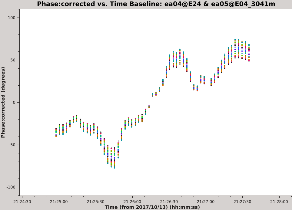
Looking at the output of listobs we see that there is a long scan on the amplitude calibrator, 3C286 (field ID 2). A feature of the VLA CASA pipeline is that it only applies scan-averaged calibration solutions to the calibrator fields, so it will not have corrected for any variations within a scan. We will plot the calibrated phase vs. time for a single antenna, paging by baseline:
# in CASA
plotms(vis='17B-197.sb34290063.eb34589992.58039.86119096065.ms', xaxis='time', yaxis='phase', ydatacolumn='corrected', field='2', antenna='ea05', correlation='RR,LL', avgchannel='64', iteraxis='baseline', coloraxis='spw')
- vis='17B-197.sb34290063.eb34589992.58039.86119096065.ms' : To plot visibilities from the pipeline calibrated MS.
- xaxis='time', yaxis='phase' : To set time as the x-axis and phase as the y-axis of the plot.
- ydatacolumn='corrected' : To plot the calibrated data (from the CORRECTED_DATA column).
- field='2' : To select visibilities from field ID 2, i.e., the amplitude calibrator 3C286.
- antenna='ea05', iteraxis='baseline' : To view a single baseline at a time. Any single antenna can be chosen here.
- correlation='RR,LL' : To plot both parallel-hand correlation products.
- avgchannel='64' : To average all channels in each SPW to increase signal-to-noise. Since the bandpass solutions have been applied to these data the channels will average coherently.
- coloraxis='spw' : To plot each SPW as a different color, which will make it easier to distinguish them.
Use the 'Next Iteration' button of the plotms GUI to cycle through additional baselines. You should see plots that look similar to the example image of the ea04-ea05 baseline (see Figure 1). The plotted data have a mean of zero phase because the pipeline calibration solutions have already been applied. The phase is seen to vary with time over a large range (in some cases more than +/- 100 degrees) and the variations appear to be smooth over time scales of a few integrations. For a given baseline, we can see that all of the spectral windows and both correlations approximately follow the same trend with time. Additionally, the magnitude of the phase variations is larger for the higher frequency spectral windows, a pattern that is consistent with changes in atmospheric density.
Optional extra steps: Create and inspect similar plots using scan 2 of the phase calibrator field (J1549+5038). Repeat for baselines to other antennas.
Splitting the Target Visibilities
CASA calibration tasks always operate by comparing the visibilities in the DATA column to the source model, where the source model is given by either the MODEL_DATA column, a model image or component list, or the default model of a 1 Jy point source at the phase center. For example, the calibration pipeline used the raw visibilities in the DATA column to solve for calibration tables and then created the CORRECTED_DATA column by applying these tables to the DATA column. With this context in mind, an essential step for self-calibration is to split the calibrated visibilities for the target we want to self-calibrate, meaning that the visibilities of the target source get copied from the CORRECTED_DATA column of the pipeline calibrated MS to the DATA column of a new measurement set. Self-calibration will work in the same way as the initial calibration, i.e., by comparing the pipeline calibrated visibilities (which are now in the DATA column of the new split MS) to a model, solving for self-calibration tables, and then creating a new CORRECTED_DATA column by applying the self-calibration tables. If we did not split the data, we would need to constantly re-apply all of the calibration tables from the pipeline (both on-the-fly when computing the self-calibration solutions and then again when applying the self-calibration), which would make the process much more cumbersome.
# in CASA
split(vis='17B-197.sb34290063.eb34589992.58039.86119096065.ms', datacolumn='corrected', field='1', correlation='RR,LL', outputvis='obj.ms')
- vis='17B-197.sb34290063.eb34589992.58039.86119096065.ms' : The input visibilities for split. Here, these are the visibilities produced by the pipeline.
- datacolumn='corrected' : To copy the calibrated visibilities from the input MS.
- field='1' : The field ID of the target we want to self-calibrate.
- correlation='RR,LL' : To select only the parallel hand correlations. This will make the output data set smaller by about a factor of two.
- outputvis='obj.ms' : The name of the new measurement set that split will create.
The Initial Model
Now that we understand the data a bit better and know that we need to apply self-calibration, we will begin to work our way through the steps outlined in the Introduction (create initial model, create calibration table, inspect solutions, determine best solution interval, applycal, split, next round). We first begin with creating an initial model which gaincal will compare to the data in order to create the calibration table that will be applied to the data in the first round of self-calibration.
Preliminary Imaging
Prior to solving for self-calibration solutions we need to make an initial model of the target field, which we will generate by deconvolving the target field using the task tclean. There are several imaging considerations that we should address when making this model (discussed below). See the VLA CASA Guide on Imaging for more details about these parameters.
Image field-of-view: Ideally, we want our self-calibration model to include all of the sources present in the data (e.g., sources near the edge of the primary beam or in the first sidelobe). This is typically achieved by making an image large enough to encompass all of the apparent sources, or by making a smaller image of the target plus one or more outlier fields. We will start with a large dirty image of the entire primary beam (PB) in order to better understand the sources in the galaxy cluster plus any background sources that will need to be cleaned. A rule of thumb for the VLA is that the FWHM of the PB in arcminutes is approximately 42 * (1 GHz / nu). At the center frequency of our C-band observations (5.5 GHz) the VLA primary beam is ~8' FWHM. In order to image the entire PB and the first sidelobe we need an image field of view that is about four times larger, so we will choose a 32' field-of-view for our initial image (see Wide-Field-Imaging (CASAdocs) and Field-of-View (VLA OSS) for further discussion of primary beams).
Primary beam mask: By default, the 'pblimit' parameter will add an image mask everywhere the value of the primary beam is less than 20%. We want to turn off this mask, as it would prevent us from viewing the image over our desired field of view. This mask is turned off by setting the magnitude of the 'pblimit' parameter to be negative. The actual value of this parameter is unimportant (but do NOT use 1, -1, or 0) for the imaging we will be doing (i.e., the 'standard', 'widefield' and 'wproject' gridders).
Image cell size: There are a few different ways to estimate the synthesized beam size for these observations taken with the C-band in the B-configuration. For one, we can use the Resolution table (VLA OSS), which gives a resolution of 1.0". It is recommended to choose a cell size that will result in at least 5 image pixels across the FWHM of the synthesized beam, therefore we require a cell size of 0.20"/pixel or smaller.
Image size in pixels: We can convert our desired field-of-view to pixels using the cell size: 32' * (60" / 1') * (1 pixel / 0.20") = 9600 pixels.
Wide-field effects: Large images may require additional consideration due to non-coplanar baselines (the W-term). In CASA, this is usually addressed by turning on the W-project algorithm. See Wide-Field-Imaging (CASAdocs) for a more detailed discussion.
We can estimate whether our image requires W-projection by calculating the recommended number of w-planes using this formula taken from page 392 of the NRAO 'white book',
[math]\displaystyle{ N_{wprojplanes} = \left ( \frac{I_{FOV}}{\theta_{syn}} \right ) \times \left ( \frac{I_{FOV}}{1\, \mathrm{radian}} \right ) }[/math]
where I_FOV is the image field-of-view (32') and theta_syn is the synthesized beam size (1.0"). Working in units of arcseconds ((32 x 60) / 1.0) * ((32 x 60) / 206265) evaluates to N_wprojplanes ~ 18 so we will choose to turn on the w-project algorithm with gridder='widefield' and set wprojplanes=18. If the recommended number of planes had been <= 1 then we would not have needed to turn on the wide-field gridder, and we could have used gridder='standard' instead.
We will now create a preliminary dirty image using these parameters.
# in CASA
tclean(vis='obj.ms', imagename='obj.dirty.9600pix', datacolumn='data', imsize=9600, cell='0.2arcsec', pblimit=-0.1, gridder='widefield', wprojplanes=18)
- datacolumn='data' : To image the visibilities in the measurement set's DATA column.
- imsize=9600: The number of pixels across one side of the (square) image.
- cell='0.2arcsec': The size of an image pixel (see above).
- pblimit=-0.1: We set this to a small negative number to turn off the PB mask, allowing us to view the entire image.
- gridder='widefield': To turn on the w-project algorithm.
- wprojplanes=18: The number of w-planes to use for w-projection.
While running tclean, you may notice a warning message that looks like this:
task_tclean::SIImageStore::restore (file casa-source/code/synthesis/ImagerObjects/SIImageStore.cc, line 2245) Restoring with an empty image model. Only residuals will be processed to form the output restored image.
This is expected when creating a dirty image. The model is blank because we haven't done any deconvolution in this tclean execution (i.e., niter=0) and we haven't started with a preexisting model (e.g., by using the 'startmodel' parameter or by resuming a previous tclean execution).
After tclean has finished, you should now open the dirty image in CARTA. On NRAO machines, open a new terminal tab, cd to the working directory, then type:
# in terminal
carta --no_browser
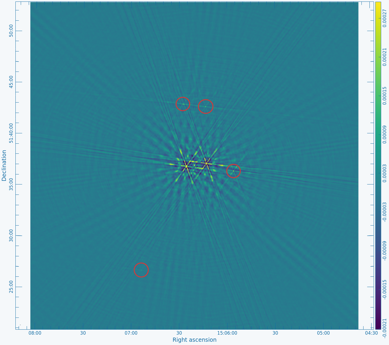
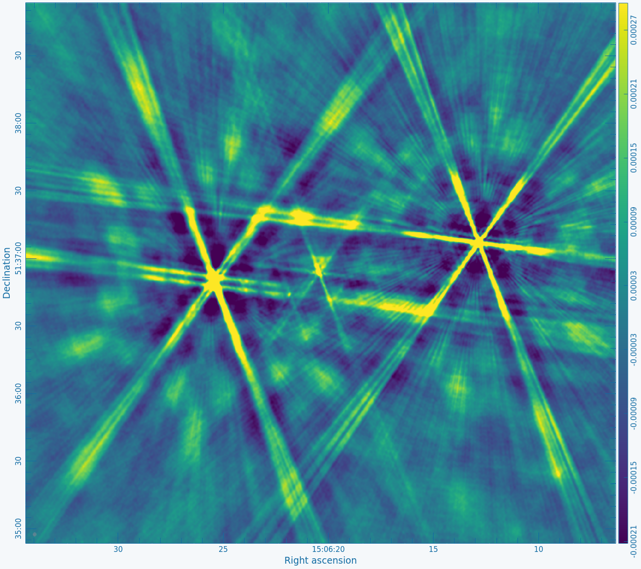
Copy the output URL into a browser to view your CARTA session. Select "obj.dirty.9600pix.image" to load. Figure 2A below shows the resulting dirty image, and Figure 2B shows a zoom-in of the central region of the image. Several outlying sources are detectable; the four brightest are marked with red circles. Use the red Min and Max sliders in the Render Configuration tool to adjust the image. Linear scaling with viridis color map is used in the below example.
 |
 |
We have a few options about how to deal with these outlying sources:
- Proceed with the self-calibration procedure using a large field-of-view that includes all the outlying sources.
- Proceed with the self-calibration procedure using a small field-of-view that includes only the central sources, and add an outlier field on each of the outlying sources.
- Proceed with the self-calibration procedure using a small field-of-view that includes only the central sources, ignoring the outlying sources.
In this guide, we will first choose to ignore the outlying sources in order to present a simplified self-calibration procedure. This is also what was chosen for the scientific image and analysis because the artifacts from the outlying sources did not strongly effect the area of scientific interest (inner 3'). For more information about the other options described above, see the VLA Imaging CASAguide and the tclean task documentation. Sometimes, more advanced techniques are used for outlying sources such as UV-subtraction, peeling or direction-dependent calibration, but these are outside the scope of this guide.
Creating the Initial Model
After deciding how to deal with the outlying sources, our next step is to make the initial model that we will use for self-calibration. There are a few additional parameters that apply to this step, discussed below.
Image field-of-view: For this science case we are only interested in sources within ~1.5' radius of the cluster center. Since we have chosen to ignore the outlying sources at this stage, we will proceed with an image field-of-view of 3'.
Wide-field effects: We repeat the calculation of wprojplanes from the Initial Imaging section using our new field of view of 3'. This results in wprojplanes ~ 1 so we turn off the correction for non-coplanar baselines by setting gridder='standard'.
Wide-band imaging: Our images will combine data from all spectral windows, spanning a frequency range of about 4.5-6.5 GHz (a fractional bandwidth of about 36%). Each source's amplitude may vary substantially over this frequency range, due to either the source's intrinsic spectral variation and/or the frequency dependence of the VLA's primary beam. To mitigate these errors during deconvolution we will use deconvolver='mtmfs' and nterms=2. For further discussion of wide-band imaging, see Wide-Band-Imaging (CASA docs) and the VLA Imaging CASAguide.
Image deconvolution: We will need to deconvolve (clean) this image in order to produce a model of the field. We will want to control the cleaning depth and masking interactively, so we set interactive=True. We also must choose the number of clean iterations with the niter parameter. A suggested starting value is niter=1000 iterations, but this can be changed interactively after we start cleaning.
Imaging weights: When constructing the initial model, especially when there are large image artifacts, it is recommended to use "robust" imaging weights. In CASA, this is enabled with weighting='briggs', and then choosing a value for the robust parameter between -2 and +2. Values of robust near +2 (approximately natural weighting) often result in large positive PSF sidelobes while robust near -2 (approximately uniform weighting) often produce large negative PSF sidelobes. Since many types of image artifacts scale with PSF sidelobe levels, a reasonable compromise is often around robust=0.
Saving the model: After deconvolution, there are a couple options for how to write the model back to the measurement set, controlled by the savemodel parameter. The default is none which will not save the model. It is essential that this default is changed or else the selfcal procedure will not work properly. The option savemodel='virtual' will save a copy of the image to the SOURCE subtable of the measurement set to be used later for on-the-fly model visibility prediction. This option is sometimes recommended for very large data sets, but is not generally recommended. The other option, savemodel='modelcolumn' is the recommended setting and the one that we will use in this guide. This option will predict the model visibilities after cleaning and save the result to the MODEL_DATA column.
Now we are ready to create our first clean image. This image will provide the starting model that is required by the calibration routines, and it will showcase why we need self-calibration for these data.
# in CASA
tclean(vis='obj.ms', imagename='obj.prelim_clean.3arcmin', datacolumn='data', imsize=900, cell='0.2arcsec', pblimit=-0.1, gridder='standard', deconvolver='mtmfs', nterms=2, niter=1000, interactive=True, weighting='briggs', robust=0, savemodel='modelcolumn')
- datacolumn='data' : To image the visibilities in the measurement set's DATA column.
- imsize=900: To create an image with a 3' field-of-view.
- cell='0.2arcsec': The size of an image pixel.
- pblimit=-0.1: To remove the PB mask; see previous sections.
- gridder='standard': We select the default gridder (assumes coplanar baselines).
- deconvolver='mtmfs': We will turn on the wide-band deconvolution algorithm as discussed above.
- nterms=2: The number of Taylor terms for wide-band deconvolution.
- niter=1000: Set a relatively large number of iterations as a starting point.
- interactive=True: So we can interactively place the mask.
- weighting='briggs': Turn on 'robust' image weighting
- robust=0: Set the value of the robust weighting.
- savemodel='modelcolumn': To enable writing the MODEL_DATA column to the MS after imaging. **important**
Interactive tclean will open the image in a CASA viewer window. Select All Channels and All Polarizations. Then, place conservative circular masks around each of the strong sources in turn, starting with the brightest:
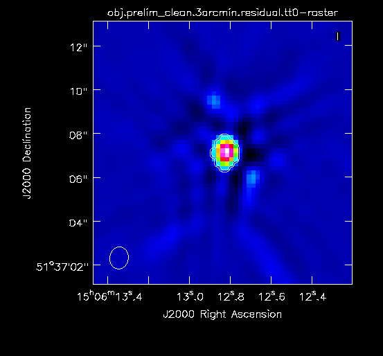
- First mask the rightmost source (Figure 3A), press the green circle arrow in the CASA viewer to perform one cycle of cleaning, and wait for focus to return to the viewer. The viewer will then show you the current residual image (i.e., the image after subtracting some flux from within the first mask).
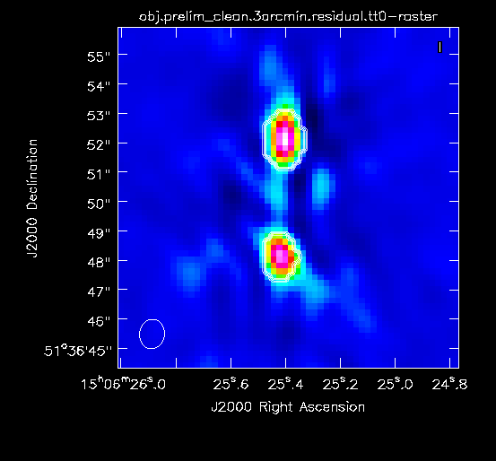
- Then mask the leftmost double-lobed source (Figure 3B) and press the green circle arrow in the CASA viewer. This will perform the next cleaning cycle, after which focus will return to the viewer. Cleaning has now taken place inside the masks of both sources and the brightest source in the new residual image will be in the middle.
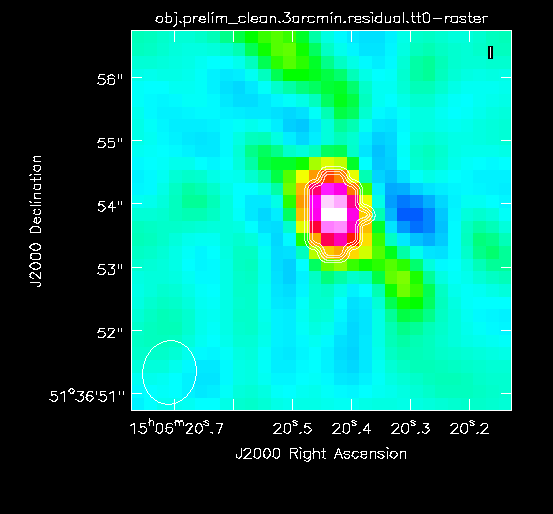
- Finally, mask the middle source (Figure 3C), press the green circle arrow again, and wait for CASA to complete the next cycle of cleaning.
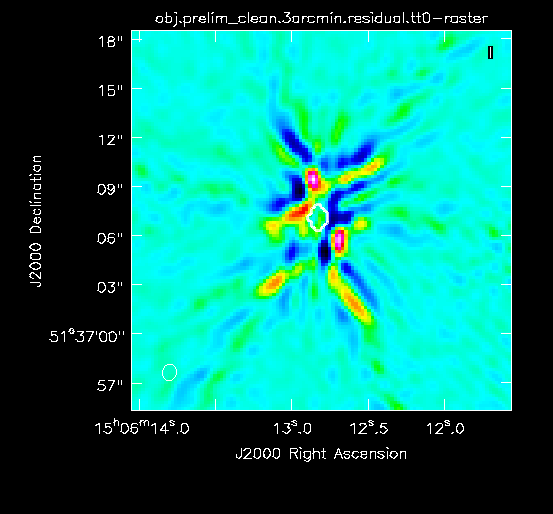
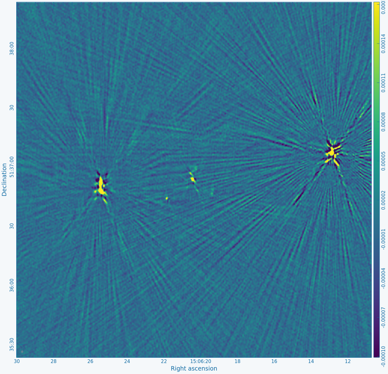
At this point, the residual emission is at about the same level as the artifacts so we stop cleaning (press the red X in the CASA viewer; see Figure 3D for an example of the artifacts). It is strongly recommended to only mask and clean emission that is believed to be real so as not to include artifacts in the model.
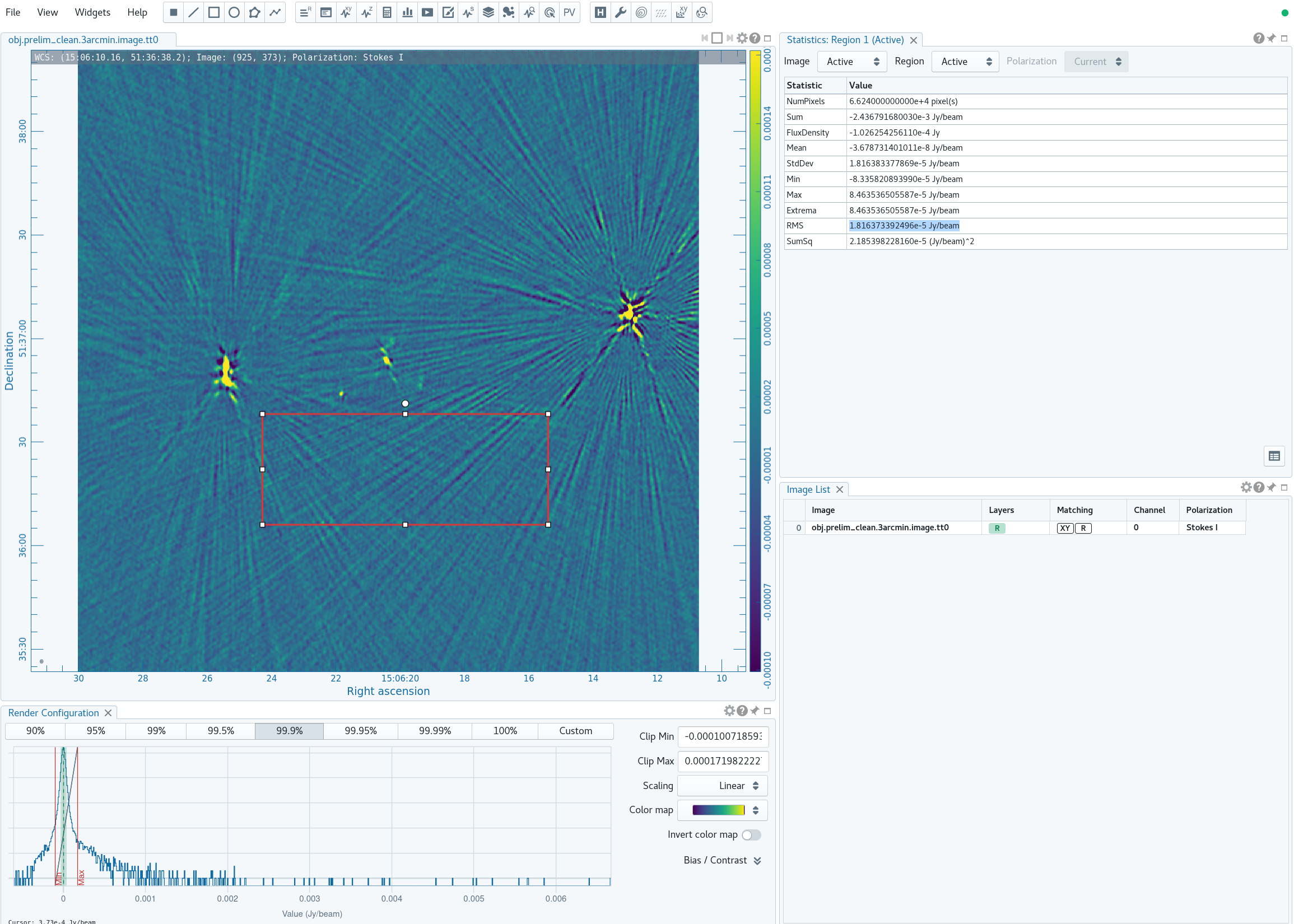
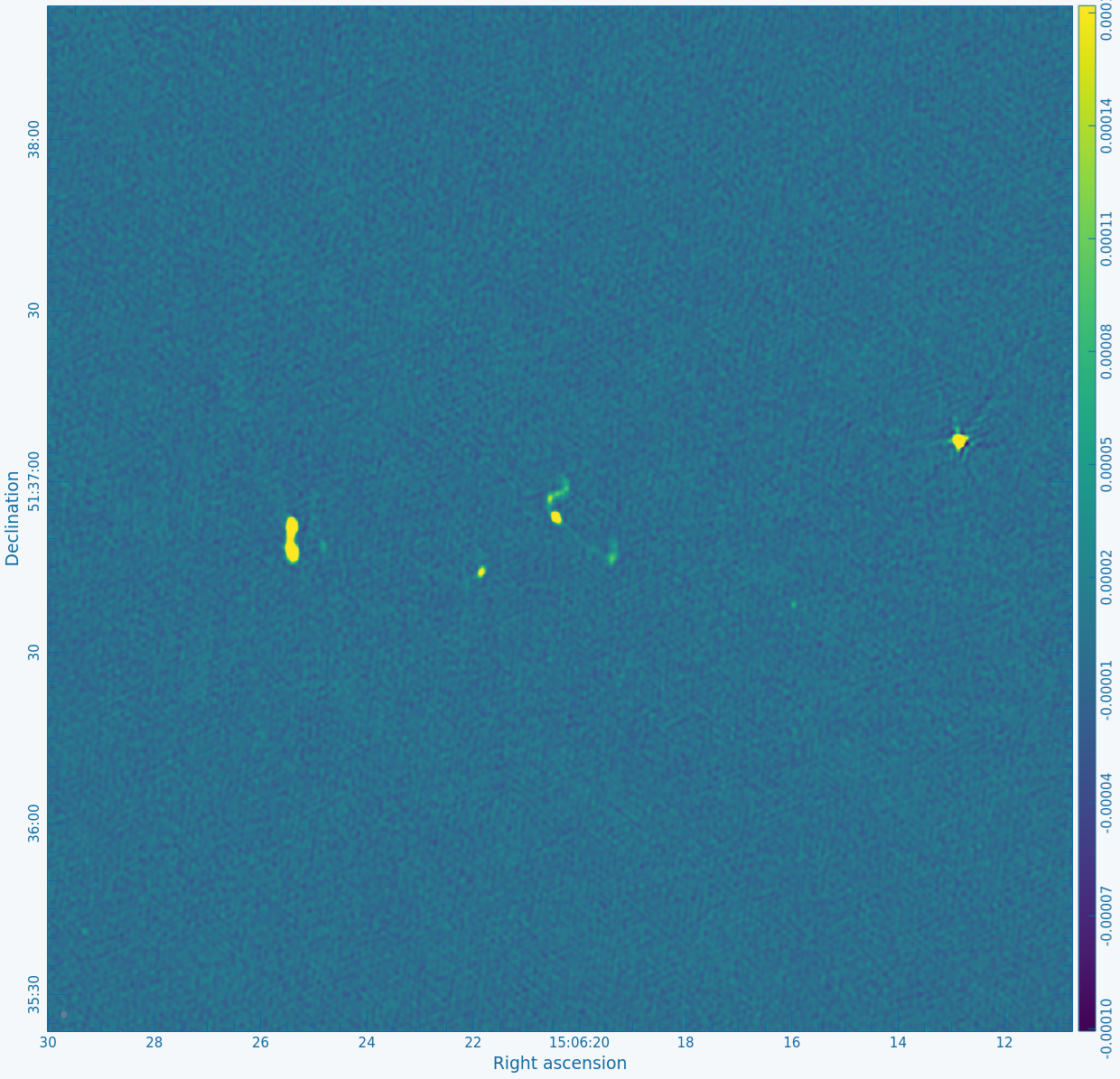
Now in CARTA we will examine the resulting clean image (obj.prelim_clean.3arcmin.image.tt0; see Figure 4A) that we will try to improve through the use of self-calibration. For reference, we will measure some simple image figures of merit to compare with the image after self-calibration. Open the Statistics Widget (calculator symbol). Specifically, we measure the peak intensity (Max) in the image to be 6.67 mJy. Now draw a large region that does not contain a source (see Figure 4B). The statistics widget displays the image noise (RMS) of the active region to be 18.2 uJy. This gives a ratio between the maximum and the noise of 366, which is called the dynamic range.
Verifying the Initial Model
There have been reported instances where CASA fails to save the model visibilities when using interactive clean. It is crucial that the model is saved correctly, otherwise self-calibration will use the 'default' model of a 1 Jy point source at the phase center. The default model may be very different from your target field and we do not want to carry out the self-cal procedure with this incorrect model. Therefore, it is recommended to verify that the model has been saved correctly by inspecting the model visibilities.
# in CASA
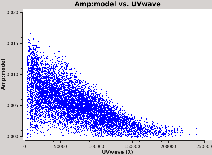
plotms(vis='obj.ms', xaxis='UVwave', yaxis='amp', ydatacolumn='model', avgchannel='64', avgtime='300')
- vis='obj.ms' : To plot visibilities from the split MS.
- xaxis='UVwave', yaxis='amp' : To set UV-distance in wavelengths as the x-axis and amplitude as the y-axis of the plot.
- ydatacolumn='model' : To plot the model visibilities (from the MODEL_DATA column).
- avgchannel='64' : To average all channels per SPW.
- avgtime='300' : To average in time in chunks of 300 seconds.
The resulting plot should resemble Figure 5 on the right. This plot shows that some baselines see up to 15 mJy of flux, but that the source becomes resolved on the longer baselines. Note that the visibilities plotted here are for correlations RR and LL since we dropped RL and LR with the split task. However, had we retained RL and LR, they would equal zero since we only made a Stokes I model image.
This model that has been plotted is clearly not the default model of a 1 Jy point source (if it was, all amplitudes would be at 1 Jy) and so we have verified that tclean has correctly written the MODEL_DATA column of the MS.
First Round of Self-Calibration
Solving for the First Self-Calibration Table
For this first round of selfcal we will use the model that we just created above and compare it to the data in order to create a table of corrections to apply to the data. We are now ready to solve for these first selfcal solutions. We will explore various parameters of the task gaincal in order to learn more about the data and settle on the optimal parameters. The most relevant parameters are discussed below:
Solution interval: This is controlled with the solint parameter and is one of the most fundamental parameters for self-calibration. The value of this parameter can vary between 'int' which stands for integration and will be the time of a single integration for that data set (corresponding to 3 seconds for this data set) up to 'inf' for infinite (meaning either an entire scan or the entire observation, depending on the value of the combine parameter). We typically want to choose the shortest solution interval for which we can achieve adequate signal-to-noise in the calibration solutions.
Data combination: The data can be combined in multiple ways to improve signal-to-noise, but if the target source is bright enough to obtain good calibration solutions in a short timescale without data combination, then these options are not necessary. However, if low signal-to-noise messages appear across antennas, times, and SPWs, then both parallel-hand correlations, if present, can be combined by setting gaintype='T' instead of gaintype='G' , and this will generally increase the signal-to-noise by an additional factor of root 2. If gaincal still produces a lot of low signal-to-noise messages, one can try to combine multiple SPWs with combine='spw' if the SPWs are at similar frequencies, and can generally expect to increase the solution's signal-to-noise by the square root of the number of SPWs that are combined. Combining scans during self-calibration is not usually recommended.
Amplitude and phase correction: Because large phase errors will result in incoherent averaging and lead to lower amplitudes, we always want to start with phase-only self-calibration. We achieve this by setting calmode='p' . In later rounds of selfcal, after the phases have been well corrected, we can try calmode='ap' to include an amplitude component in the solutions. When solving for amplitudes, we may also want to consider normalizing them with the solnorm parameter.
Reference antenna: As with standard calibration, we want to choose a reference antenna for the calibration solutions. It is generally recommended to choose one that is near the center of the array but not heavily flagged. In order to determine which one to use, use plotants to plot the positions of the antennas and choose one near the center. To find the percent data flagged per antenna, you could run flagdata with mode='summary'.
Signal-to-noise ratio (SNR): The default minimum SNR in gaincal is 3.0, but this can be adjusted with the minsnr parameter. Solutions below this minimum are flagged in the output calibration table. Sometimes we want to increase this minimum, e.g., to 5.0, to reject noisy solutions. Alternatively, we may want to lower this minimum, e.g., to zero, usually for inspection purposes.
We will now create our initial self-calibration table. This will not be the final table for the first round of self-calibration, but rather, a temporary table that we will inspect to help determine the optimal parameters.
# in CASA
gaincal(vis='obj.ms', caltable='selfcal_initial.tb', solint='int', refant='ea24', calmode='p', gaintype='G', minsnr=0)
- caltable='selfcal_initial.tb': Name the calibration tables something intuitive to distinguish each one.
- solint='int': We choose a solution interval equal to the integration time (3 seconds) in order to get a sense of the structure and timescale of the variations.
- refant='ea24': The chosen reference antenna.
- calmode='p': To start with phase only calibration.
- gaintype='G': To solve for the polarizations separately.
- minsnr=0: To turn off flagging of low-SNR solutions, so that we can inspect all the solutions.
You may see several messages printed to the terminal while gaincal is running, e.g.,
Found no unflagged data at: (time=2017/10/13/20:50:07.5 field=0 spw=0 chan=0)
This means that all the input data was flagged for this solution interval. This is generally harmless unless there are far fewer solutions in the output table than you were expecting.
It is recommended to check the logger messages written by gaincal to find the total number of solution intervals, i.e.,
INFO gaincal	Calibration solve statistics per spw:  (expected/attempted/succeeded):
INFO gaincal	  Spw 0: 561/522/522
INFO gaincal	  Spw 1: 561/522/522
...  ...          ...
This shows that gaincal successfully found solutions for most of the solution intervals.
Plotting the First Self-Calibration Table
To view these solutions, we use plotms.
# in CASA
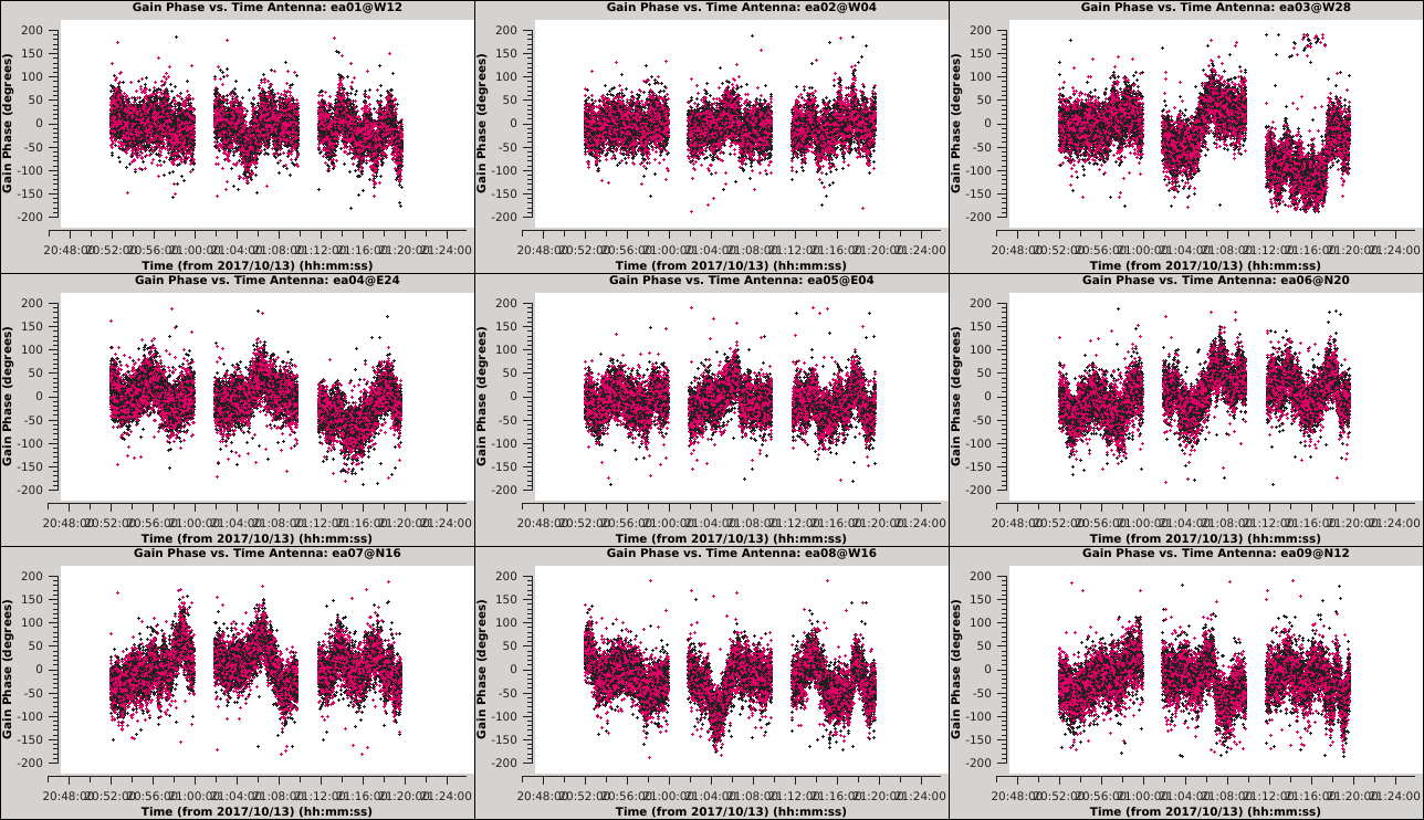
plotms(vis='selfcal_initial.tb', xaxis='time', yaxis='phase', iteraxis='antenna', gridrows=3, gridcols=3, coloraxis='corr')
- xaxis='time' & yaxis='phase' : View the phase variations over time with respect to antenna 24.
- iteraxis='antenna' : Create separate plots of the corrections for each antenna.
- gridrows=3 & gridcols=3: It can be helpful to view multiple plots at once, as we will be stepping through several plots. In this case, 9 plots per page.
- coloraxis='corr' : To use different colors when plotting different polarizations (R and L will be black and red, respectively).
Iterate through these plots using the 'Next Iteration' button (green triangle) to inspect the solutions for all antennas. Some noteworthy observations include:
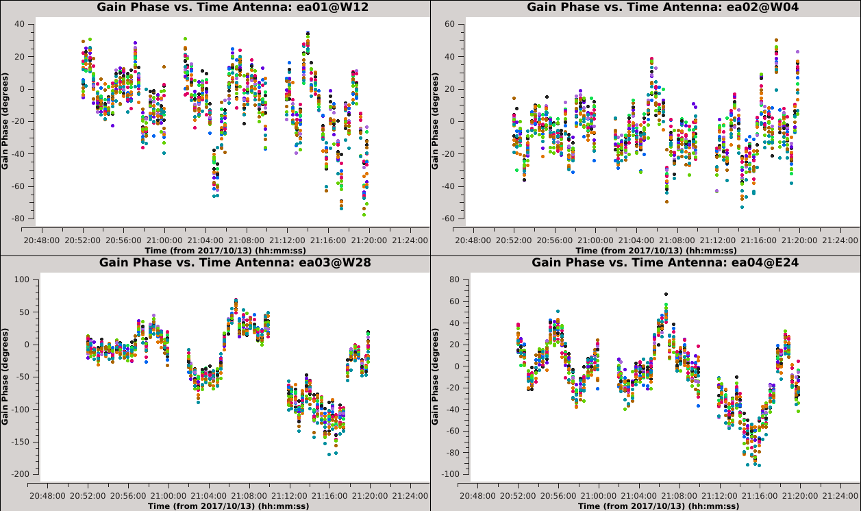
- There are large, coherent phase changes of more than 100 degrees.
- The timescale of these changes is fairly short, about 20 seconds (zoom in on the variations for a particular antenna to see this).
- The scatter in these signals is high (approximately a few 10s of degrees), indicating low signal-to-noise.
- The phase changes in the two polarizations appear to match each other.
- There is some interesting behavior in the 3rd scan for antennas ea15 and ea27.
Note: The plot of the reference antenna, ea24, is not unusual and should be considered to be consistent with zero phase.
It is apparent from these plots that we can combine polarizations to improve the solution signal-to-noise ratio, since we observed that the solutions for the two polarizations were very similar.
The next thing we want to understand is if we can combine SPWs, and if so, which ones. We can plot the previous solutions in a slightly different way to help answer this question. We will view these solutions again using plotms, but this time we will color the solutions by SPW.
# in CASA
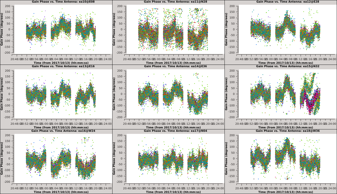
plotms(vis='selfcal_initial.tb', xaxis='time', yaxis='phase', iteraxis='antenna', gridrows=3, gridcols=3, coloraxis='spw')
Iterate again through these plots using the 'Next Iteration' button (green triangle) to inspect the solutions for all antennas. When you get to ea15, it should be clear that the solutions are not the same for all SPWs. This is also true but less obvious for ea27 due to the limited number of colors available to plotms.
We can inspect this further in the following plot:
# in CASA
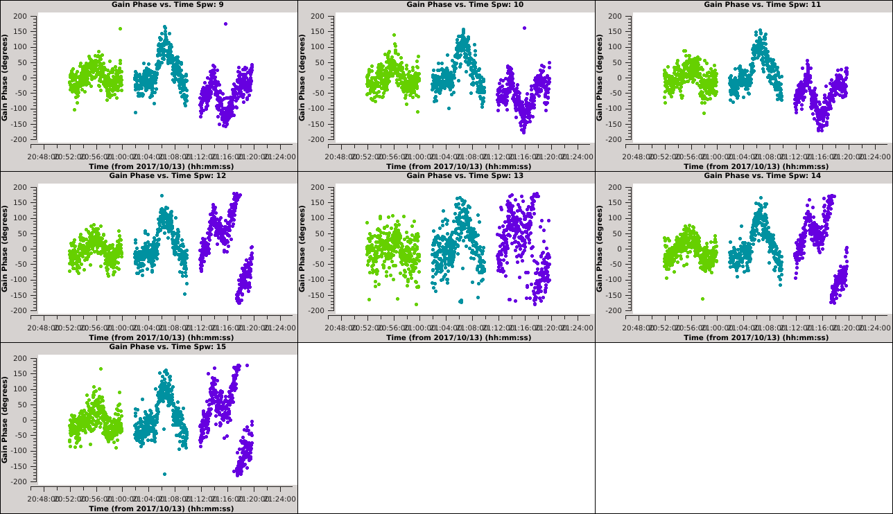
plotms(vis='selfcal_initial.tb', xaxis='time', yaxis='phase', antenna='ea15', iteraxis='spw', gridrows=3, gridcols=3, coloraxis='scan')
- antenna='ea15' : To select only antenna ea15.
- iteraxis='spw' : Create separate plots of the corrections for each SPW.
- coloraxis='scan' : To use different colors when plotting different scans.
The first set of 9 plots should have a similar pattern. On the next iteration, this pattern should continue for SPWs 9~11, but then change for SPWs 12~15. The signal-to-noise for SPW 13 is also noticeably lower. If we create these plots for ea27, we will see a similar pattern, only this time the pattern is constant over SPWs 0~5 and then changes to a new pattern that is constant for SPWs 6~15. For both ea15 and ea27, the change only happens in the third of the three scans.
Unfortunately, since all SPWs do not show the same phase solutions, it will not be trivial to combine them to increase the signal-to-noise ratio of the solutions. Therefore, we will continue without combining SPWs.
Examples of Various Solution Intervals
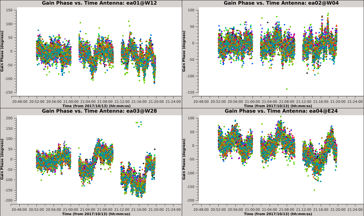
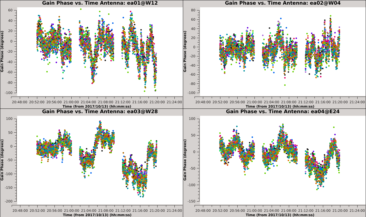
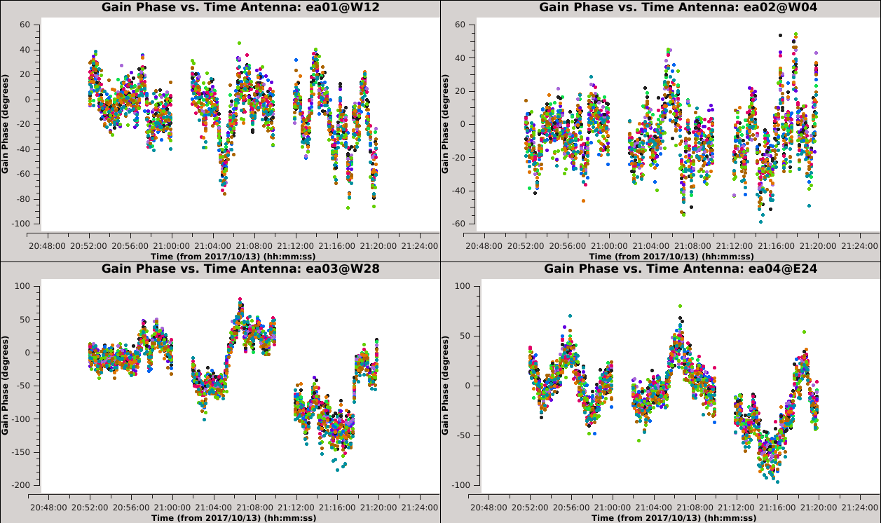
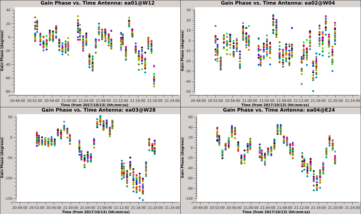
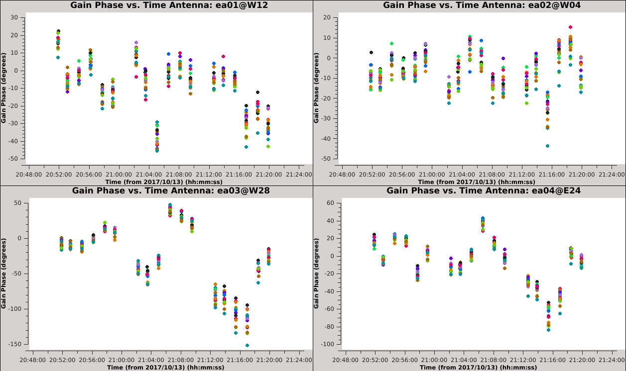
Now that we have made the decision about how to handle SPW combination, we will move on to consider time averaging. We observed the previous solutions to display large, coherent phase changes, but also to have significant scatter due to low signal-to-noise. We could increase the signal-to-noise by root 2 for each doubling of the solution interval, but it does not make sense to average over timescales larger than the characteristic time over which the phase remains constant (approximately 20 seconds for these data). In this section, we will demonstrate these effects by creating and plotting tables over a range of solution intervals. We will also combine both polarizations (with gaintype='T' ) to improve the solution signal-to-noise ratio, since we observed the two polarizations to measure approximately the same phase changes.
These commands will create 6 new tables having solution intervals of 3, 6, 12, 24, 48 and 96 seconds (1, 2, 4, 8, 16 and 32 times the data's integration time). The commands can all be entered together and will take a while to run.
# in CASA
gaincal(vis='obj.ms',caltable='selfcal_combine_pol_solint_3.tb',solint='int',refant='ea24',calmode='p',gaintype='T', minsnr=0)
gaincal(vis='obj.ms',caltable='selfcal_combine_pol_solint_6.tb',solint='6s',refant='ea24',calmode='p',gaintype='T', minsnr=0)
gaincal(vis='obj.ms',caltable='selfcal_combine_pol_solint_12.tb',solint='12s',refant='ea24',calmode='p',gaintype='T', minsnr=0)
gaincal(vis='obj.ms',caltable='selfcal_combine_pol_solint_24.tb',solint='24s',refant='ea24',calmode='p',gaintype='T', minsnr=0)
gaincal(vis='obj.ms',caltable='selfcal_combine_pol_solint_48.tb',solint='48s',refant='ea24',calmode='p',gaintype='T', minsnr=0)
gaincal(vis='obj.ms',caltable='selfcal_combine_pol_solint_96.tb',solint='96s',refant='ea24',calmode='p',gaintype='T', minsnr=0)
These commands will plot each of the newly created tables. Run the commands sequentially (or simply change the selected table in Data > Browse, then click Plot to update) and use the plotms GUI to iterate through the plots of additional antennas.
# in CASA
plotms(vis='selfcal_combine_pol_solint_3.tb',yaxis='phase',iteraxis='antenna',gridrows=2, gridcols=2, coloraxis='spw')
plotms(vis='selfcal_combine_pol_solint_6.tb',yaxis='phase',iteraxis='antenna',gridrows=2, gridcols=2, coloraxis='spw')
plotms(vis='selfcal_combine_pol_solint_12.tb',yaxis='phase',iteraxis='antenna',gridrows=2, gridcols=2, coloraxis='spw')
plotms(vis='selfcal_combine_pol_solint_24.tb',yaxis='phase',iteraxis='antenna',gridrows=2, gridcols=2, coloraxis='spw')
plotms(vis='selfcal_combine_pol_solint_48.tb',yaxis='phase',iteraxis='antenna',gridrows=2, gridcols=2, coloraxis='spw')
plotms(vis='selfcal_combine_pol_solint_96.tb',yaxis='phase',iteraxis='antenna',gridrows=2, gridcols=2, coloraxis='spw')
The following figures show examples of the first iteration of each of the above plots.
Comparing the Solution Intervals
We can see from plotting these solutions that the shortest timescale solutions capture the structure of the phase variations, but with a large dispersion. If we were to apply these low signal-to-noise ratio (SNR) solutions then we would, on average, be correcting for the large phase changes, but we would also introduce random phase errors that could reduce the sensitivity of our observation. Another concern with using low-SNR solutions is that they can overfit the noise in the visibilities, leading to biases in the self-calibrated image. In this guide we adopt a conservative minimum SNR of 6 in order to guard against these biases.
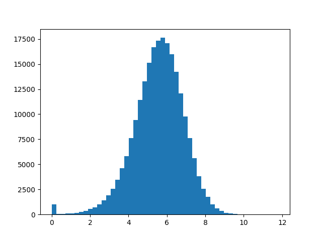
Let's take a closer look at the SNR of the table with the 3 second integration time. We will use the table toolkit (tb) to extract the SNR of each solution which will return the SNR values as a numpy ndarray (and the numpy ravel method will flatten the result into a 1-dimensional array). Then we use numpy and scipy to print some statistical quantities and matplotlib to make a histogram.
# in CASA
import numpy as np
import matplotlib.pyplot as plt
from scipy import stats

tb.open( 'selfcal_combine_pol_solint_3.tb' )
snr_3s = tb.getcol( 'SNR' ).ravel()
tb.close()

plt.hist( snr_3s, bins=50 )

print( 'median = {0}'.format( np.median( snr_3s ) ) )
print( 'P(<=6) = {0}'.format( stats.percentileofscore( snr_3s, 6 ) ) )
We can see from the output that the median SNR is about 5.6 for this table and that enforcing our desired minimum SNR of 6 would flag 62% of the solutions. We want to avoid flagging such a high fraction of solutions, so we need to consider longer solution intervals to raise the SNR.
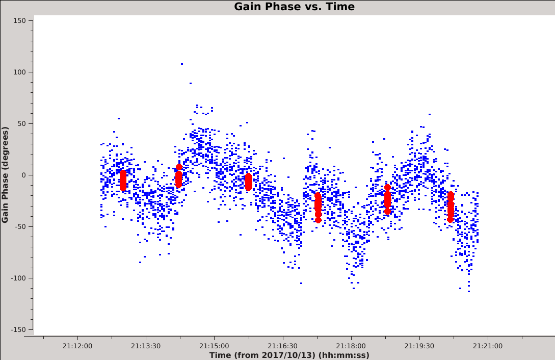
The longest solution interval in our examples (96 seconds) has a different problem. Specifically, we can see that the intrinsic phase is varying faster than the solution interval, so the solutions no longer do a good job of capturing the changes that we are trying to correct for. Applying such long timescale solutions may lead to some improvement in the image, but we would be leaving residual phase errors in the corrected data. This is particularly obvious if we overplot the solutions using plotms. The figure to the right shows one such example, created with the following two commands:
# in CASA
plotms('selfcal_combine_pol_solint_3.tb', antenna='ea01', scan='7', yaxis='phase')

plotms('selfcal_combine_pol_solint_96.tb', antenna='ea01', scan='7', yaxis='phase', plotindex=1,
clearplots=False, customsymbol=True, symbolsize=12, symbolcolor='ff0000', symbolshape='circle')
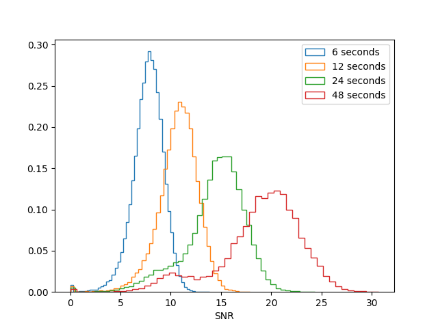
Given these considerations, we suggest that the optimal selfcal parameters will use the shortest possible interval for which the signal-to-noise is also sufficient. Having identified shortcomings with the shortest (3s) and longest (96s) solution intervals in our set of example tables, we will now take a closer look at the SNR of the intermediate tables. The following code will compare the SNR histograms and compute the fraction of solutions less than a SNR of 6. You may need to close the previous SNR plot (Figure 10) for the new plot to open correctly.
# in CASA

tb.open( 'selfcal_combine_pol_solint_6.tb' )
snr_6s = tb.getcol( 'SNR' ).ravel()
tb.close()

tb.open( 'selfcal_combine_pol_solint_12.tb' )
snr_12s = tb.getcol( 'SNR' ).ravel()
tb.close()

tb.open( 'selfcal_combine_pol_solint_24.tb' )
snr_24s = tb.getcol( 'SNR' ).ravel()
tb.close()

tb.open( 'selfcal_combine_pol_solint_48.tb' )
snr_48s = tb.getcol( 'SNR' ).ravel()
tb.close()

plt.hist( snr_6s, bins=50, density=True, histtype='step', label='6 seconds' )
plt.hist( snr_12s, bins=50, density=True, histtype='step', label='12 seconds' )
plt.hist( snr_24s, bins=50, density=True, histtype='step', label='24 seconds' )
plt.hist( snr_48s, bins=50, density=True, histtype='step', label='48 seconds' )
plt.legend( loc='upper right' )
plt.xlabel( 'SNR' )

print( 'P(<=6) = {0}  ({1})'.format( stats.percentileofscore( snr_6s, 6 ), '6s' ) )
print( 'P(<=6) = {0}  ({1})'.format( stats.percentileofscore( snr_12s, 6 ), '12s' ) )
print( 'P(<=6) = {0}  ({1})'.format( stats.percentileofscore( snr_24s, 6 ), '24s' ) )
print( 'P(<=6) = {0}  ({1})'.format( stats.percentileofscore( snr_48s, 6 ), '48s' ) )
These results show that imposing a minimum SNR of 6 on the 6 second table will flag more than 11% of the solutions and that the same restriction will flag less than 2% of the 12 second table's solutions. Based on these numbers, we conclude that the 12 second table provides a reasonable compromise between time resolution and signal-to-noise.
We now need to reproduce this table to impose our desired minimum SNR condition of 6.
# in CASA
gaincal(vis='obj.ms', caltable='selfcal_combine_pol_solint_12_minsnr_6.tb', solint='12s', refant='ea24', calmode='p', gaintype='T', minsnr=6)
You may see messages printed to the terminal during the gaincal execution about solutions being flagged, e.g.,
3 of 27 solutions flagged due to SNR < 6 in spw=0 at 2017/10/13/20:59:21.0
This is telling us how many solutions have been flagged for being below the minimum signal-to-noise ratio set by the minsnr parameter. You will not have seen these messages in the first execution of gaincal because we set minsnr=0, but you are likely to see them in subsequent executions now that minsnr=6. One such message is printed per-SPW and per-solution interval (time bin) if one or more of the solutions is flagged. In our example, there are 27 total solutions (one per antenna), but if we had not elected to combine polarizations there would be 56 total solutions (one per-antenna per-polarization). If you see a large number of these messages, it can be useful to try to determine if they correspond to the same antenna, SPW or time as this may indicate the presence of bad data. If these messages appear across antennas, times and SPWs then this likely indicates that the signal-to-noise is too low and that more data needs to be combined (see above recommendations in data combination).
Applying the First Self-Calibration Table
Now that we have converged on a table of self-calibration solutions we are ready to apply these to our data. The default applycal parameters are adequate to apply this table.
# in CASA
applycal(vis='obj.ms', gaintable='selfcal_combine_pol_solint_12_minsnr_6.tb')
Note: If you decide to apply solutions that you created by combining all the spectral window together (combine='spw'), then in applycal you will have to set spwmap=[0 x number of spectral windows] in order to tell CASA to apply the combined solution to all of the spectral windows. In this case, spwmap = [0,0,0,0,0,0,0,0,0,0,0,0,0,0,0,0].
Check the CASA Logger to confirm the amount of data flagged in this stage. You will see a message like:
INFO applycal T Jones: In: 86701414 / 403273728 (21.4993955669%) --> Out: 97559200 / 403273728 (24.1918065141%) (selfcal_combine_pol_solint_12_minsnr_6.tb)
This means that 21.5% of the data were already flagged prior to running applycal, and that a total of 24.2% of data are now flagged after application of the self-calibration solutions. This is reasonable, given our previous calculation of 1.8% flagged solutions, and since the percentages reported in the logger are based on counting baseline-based flags.
Another important line from the CASA Logger to pay attention to is this one:
INFO FlagVersion Creating new backup flag file called applycal_1
This is telling you that a copy of the initial (21.5%) flags was saved. You can restore the initial state of the flags using the task flagmanager should you ever wish to undo this step.
Summary of First Round of Self-Calibration
1) Create a calibration table with solint='int' and minsnr=0. Inspect the solutions, focusing on the timescale of the phase variations. 2) Create several calibration tables using multiples of the integration time. 3) Inspect these tables and choose one that balances SNR and capturing the real variations in the phase. 4) Apply chosen solution.
Imaging the Self-calibrated Data
The next thing that you may want to do is create a new image to assess the effects of the first round of self-calibration. We can do this by running tclean using similar parameters as used previously, with two notable exceptions: (1) we instruct tclean to read visibilities from the CORRECTED_DATA column since that is the column to which the self-calibration solutions have been applied, and (2) we turn off saving of the model visibilities as to not overwrite the current MODEL_DATA column.
# in CASA
tclean(vis='obj.ms', imagename='obj.selfcal1_clean.3arcmin', datacolumn='corrected', imsize=900, cell='0.2arcsec', pblimit=-0.1, gridder='standard', deconvolver='mtmfs', nterms=2, niter=1000, interactive=True, weighting='briggs', robust=0, savemodel='none')
- datacolumn='corrected' : To image the visibilities in the measurement set's CORRECTED_DATA column.
- savemodel='none': To disable writing the MODEL_DATA column.
Select All Channels and All Polarizations. During the interactive cleaning, we will again place circular masks around each of the strong sources. First we mask the rightmost source and click the green arrow. Comparing the sidelobe pattern around the rightmost source with Figure 3A, you may notice that the pattern is now more symmetric. This is a good sign that the deconvolution will improve. When focus returns to the viewer window, mask the leftmost double-lobed source and click the green arrow. Compare this source with Figure 3B and you will notice a similar improvement. When focus returns to the viewer, proceed to mask the central source. Also check on the masks of the first two sources. Depending on how you drew the mask for the leftmost source, you may want to enlarge the mask to include additional, low-level emission. Then click the green arrow.
We have now reached the point where we stopped the cleaning of the initial image, because the residual image appeared to be dominated by artifacts and noise. This is clearly not the case for this self-calibrated image as there is more convincingly real emission that needs to be cleaned. Specifically, there is a new source about 15 arcsec to the Southeast of the central source, and the masks around the leftmost and central sources need to be expanded to include additional emission. Continue the process of cleaning and masking a couple more times until the residual image appears dominated by artifacts / noise. Then click the red X to finish cleaning.
Inspecting the Self-calibrated Image
We can compare the intial and self-calibrated images by loading them both in CARTA. We'll make use of "Raster scaling matching" to fairly compare the images.
Switching between the two images (shown below) reveals a dramatic improvement in image quality. Specifically, the artifact patterns centered on the bright sources have been almost entirely eliminated, except for the rightmost source where the artifacts have been reduced to a level that is no longer problematic for scientific analysis of the central source. This is primarily the result of improving phase calibration, and also potentially due to the extra flagging of the low SNR solutions (which may have corresponded to some bad data). Re-measuring our fundamental image statistics, we see that the peak flux has increased from 6.67 to 9.07 mJy and the image RMS has decreased from 18.2 to 8.35 uJy. This is an improvement in dynamic range of a factor of 3x, from 366 to 1086!
Possible Next Steps
The items in this section are intended to provide some guidance on how to proceed after the first round of self-calibration. Code examples are included in some subsections for added clarity. Please note that each block of code is not intended to be run sequentially. Instead, this section is intended to be treated as a decision tree.
Decide to Stop
We have now completed the first round of self-calibration and seen a dramatic improvement in image quality. The first question we want to ask is: is this good enough to meet our scientific requirements? . The pursuit of a 'perfect' looking image is typically unnecessary and may be a large time sink. Therefore, it is important to continue trying to improve the image only if absolutely necessary. If the image is usable as-is, then we should stop here. In this specific case (with the data set used in this tutorial), one round of self-calibration was enough to achieve the scientific goals (determining the morphology of the radio sources in this galaxy cluster).
Modify Image Parameters
We may want to accept that the self-calibrated data is good enough for our science requirements, but revisit the imaging parameters used to make our final image. For example, the 3 arcmin image suffers at a low level from a source outside the image's field of view (the western source circled in Figure 2A). We could address this by repeating the final imaging with an outlier field on this source or by increasing the image size until the field of view is large enough to include the source. Other parameters we might want to think about if we decide to re-image could be: using multi-scale deconvolution, changing the value of Briggs robust weighting, changing the number of terms used for wide-band deconvolution, and changing the gridder (e.g., using awproject instead of standard).
Freeze in the Self-calibration Solutions
We may want to make a copy of the self-calibrated visibilities by running the task split. The calibrated data is in the measurement set's CORRECTED_DATA column, and if we select this column with the split task, then it will place the calibrated data in the DATA column of the output MS. This can greatly reduce the size of the measurement set since two of the three large columns of visibilities (MODEL_DATA and CORRECTED_DATA) will not be present in the output MS. Running split in this manner can be a great way to archive the final self-calibrated visibilities, prepare the data for combination with other observations, prepare the data for further rounds of self-calibration, etc. Below is an example of this step.
# in CASA
split(vis='obj.ms', datacolumn='corrected', outputvis='obj_selfcal.ms')
Further Rounds of Phase-only Self-calibration
There are a few options for how to continue trying to improve the calibration with additional rounds of selfcal. Each of these options is considered to be equally valid, but there are differences in how one keeps track of the data and the solutions.
The fundamental idea behind multiple rounds of selfcal is that we can continue to create a better model and therefore solve for more accurate solutions. Think back to our initial image, which involved a shallow, conservative clean that only modeled the brightest peaks of a few sources. Now that we have improved the calibration and can clean deeper, we can make a more complete model of the field and feed this back to solve for better solutions. Typically, successive rounds of selfcal suffer from diminishing returns, wherein the first round makes the largest corrections and yields the most noticeable image improvement. However, there are cases where several rounds are necessary to obtain the desired image quality. If you are unsure if multiple rounds are needed, one approach is just to try another round and then compare the image dynamic range and artifacts to your previous result.
Option 1
This option involves running split as above to freeze in the previous self-calibration solutions. Subsequent iterations of selfcal therefore produce incremental corrections to those that have been previously applied. This has the advantage that inspection of these 2nd order corrections can be useful when deciding to continue or stop further rounds of selfcal. Specifically, if the 2nd order solutions are noise-like with no discernible structure or offsets from zero phase, then applying them to the visibilities is unlikely to improve the image.
To proceed with this variant of selfcal, simply run split as above to freeze in the first round of solutions, then proceed with split's output measurement set in the same way we used obj.ms in this guide, i.e., set the model with tclean, then run gaincal, applycal and finally tclean again to produce the round 2 self-calibrated image. Below is an example of this procedure.
# in CASA

split(vis='obj.ms', datacolumn='corrected', outputvis='obj_selfcal.ms')

tclean(vis='obj_selfcal.ms', imagename='obj.selfcal1_prelim_clean.3arcmin', datacolumn='data', imsize=900, cell='0.2arcsec', pblimit=-0.1, gridder='standard', deconvolver='mtmfs', nterms=2, niter=1000, interactive=True, weighting='briggs', robust=0, savemodel='modelcolumn')

gaincal(vis='obj_selfcal.ms', caltable='selfcal_round2.tb', solint='12s', refant='ea24', calmode='p', gaintype='T', minsnr=6)

applycal(vis='obj_selfcal.ms', gaintable='selfcal_round2.tb')

tclean(vis='obj_selfcal.ms', imagename='obj.selfcal2_clean.3arcmin', datacolumn='corrected', gridder='standard', cell='0.2arcsec', imsize=900, pblimit=-0.1, deconvolver='mtmfs', nterms=2, niter=1000, interactive=True, weighting='briggs', robust=0, savemodel='none')
Option 2
This option avoids running split and continues to work with the original measurement set, i.e., obj.ms. First run tclean to set the model, then run gaincal. Unlike Option 1, these solutions will not be incremental. Instead, you are basically re-solving for the 1st order corrections the same way as in round 1, except you are using an updated model to do so. Then you run applycal and apply the new calibration table instead of the round 1 table. Finally, run tclean again to produce the round 2 self-calibrated image. There will not be any incremental solutions to inspect to help decide when to stop, so you will need to compare the selfcal tables and/or the final image properties. Below is an example of this procedure.
# in CASA

tclean(vis='obj.ms', imagename='obj.selfcal1_prelim_clean.3arcmin', datacolumn='data', imsize=900, cell='0.2arcsec', pblimit=-0.1, gridder='standard', deconvolver='mtmfs', nterms=2, niter=1000, interactive=True, weighting='briggs', robust=0, savemodel='modelcolumn')

gaincal(vis='obj.ms', caltable='selfcal_round2.tb', solint='12s', refant='ea24', calmode='p', gaintype='T', minsnr=6)

applycal(vis='obj.ms', gaintable='selfcal_round2.tb')

tclean(vis='obj.ms', imagename='obj.selfcal2_clean.3arcmin', datacolumn='corrected', gridder='standard', cell='0.2arcsec', imsize=900, pblimit=-0.1, deconvolver='mtmfs', nterms=2, niter=1000, interactive=True, weighting='briggs', robust=0, savemodel='none')
Option 3
This option also avoids running split and continues to work with the original measurement set, but unlike Option 2, allows you to create incremental solutions. First, run tclean to set the model. Then run gaincal and use the gaintable parameter to provide a list of all previous selfcal tables. In our example, if this was round 2, we would set gaintable='selfcal_combine_pol_solint_12_minsnr_6.tb' . This would pre-apply the round 1 selfcal table and write only incremental solutions to the output table. Then run applycal and provide a list of all previous selfcal tables plus the new table created by gaincal. Finally, run tclean again to produce the next self-calibrated image. This variant shares some benefits of Options 1 and 2, but can become unwieldly if you start to build up long lists of tables after several iterations. Below is an example of this procedure.
# in CASA

tclean(vis='obj.ms', imagename='obj.selfcal1_prelim_clean.3arcmin', datacolumn='data', imsize=900, cell='0.2arcsec', pblimit=-0.1, gridder='standard', deconvolver='mtmfs', nterms=2, niter=1000, interactive=True, weighting='briggs', robust=0, savemodel='modelcolumn')

gaincal(vis='obj.ms', caltable='selfcal_round2.tb',solint='12s', refant='ea24', calmode='p', gaintype='T', minsnr=6, gaintable='selfcal_combine_pol_solint_12_minsnr_6.tb')

applycal(vis='obj.ms', gaintable=['selfcal_combine_pol_solint_12_minsnr_6.tb','selfcal_round2.tb'])

tclean(vis='obj.ms', imagename='obj.selfcal2_clean.3arcmin', datacolumn='corrected', gridder='standard', cell='0.2arcsec', imsize=900, pblimit=-0.1, deconvolver='mtmfs', nterms=2, niter=1000, interactive=True, weighting='briggs', robust=0, savemodel='none')
Amplitude Self-calibration
When phase-only selfcal is no longer able to improve the image, and if you think there are still remaining calibration errors, then you may want to try amplitude selfcal. Amplitude selfcal works fundamentally the same as the phase-only examples, except that in gaincal you change to calmode='ap' . It is important that the amplitude corrections are solved for incrementally to the phase-only corrections so as not to apply amplitude corrections that compensate for decorrelation. That means using either Option 1 or 3 described above but not Option 2. Additionally, amplitude solutions require the fitting of an extra parameter and therefore the SNR may be lower than the phase-only solutions. It is generally recommended to include amplitude normalization by setting solnorm=True, which will force the mean (or median to improve outlier rejection) gain over times and antennas to be 1.0; this will typically help to preserve the flux-density scale, especially after multiple iterations of amplitude selfcal. The calwt parameter also becomes relevant with amplitude self-calibration; see the gaincal documentation for further details.
Below is an example based on the procedure in Option 1, where we increase the solution interval to 48s to compensate for the intrinsically lower SNR.
# in CASA

split(vis='obj.ms', datacolumn='corrected', outputvis='obj_selfcal.ms')

tclean(vis='obj_selfcal.ms', imagename='obj.selfcal1_prelim_clean.3arcmin', datacolumn='data', imsize=900, cell='0.2arcsec', pblimit=-0.1, gridder='standard', deconvolver='mtmfs', nterms=2, niter=1000, interactive=True, weighting='briggs', robust=0, savemodel='modelcolumn')

gaincal(vis='obj_selfcal.ms', caltable='selfcal_amplitude.tb', solint='48s', refant='ea24', calmode='ap', solnorm=True, normtype='median', gaintype='T', minsnr=6)

applycal(vis='obj_selfcal.ms', gaintable='selfcal_amplitude.tb')

tclean(vis='obj_selfcal.ms', imagename='obj.selfcal_amplitude_clean.3arcmin', datacolumn='corrected', gridder='standard', cell='0.2arcsec', imsize=900, pblimit=-0.1, deconvolver='mtmfs', nterms=2, niter=1000, interactive=True, weighting='briggs', robust=0, savemodel='none')
Extracted Scripts for VLA Self-Calibration Tutorial
VLASelf-calibrationTutorial.tar (21 GB)
Questions about this tutorial? Please contact the NRAO Helpdesk.
Last checked on CASA Version 6.5.4
