AntennaeBand7 Imaging 6.5.4
Last checked on CASA Version 6.5.4
This guide features CARTA, the “Cube Analysis and Rendering Tool for Astronomy,” which is the new NRAO visualization tool for images and cubes. The CASA viewer (imview) has not been maintained for a few years and will be removed from future versions of CASA. We strongly recommend using CARTA, as it provides a much more efficient, stable, and feature rich user experience. A comparison of the CASA viewer and CARTA, as well as instructions on how to use CARTA at NRAO, is provided in the CARTA section of the CASA docs.
Overview
Details of these observations are provided at AntennaeBand7. This tutorial picks up where AntennaeBand7_Calibration leaves off, with fully calibrated measurement sets of the split out science target. If you wish to skip the Calibration guide, you may obtain the calibrated data Antennae_Band7_CalibratedData.tgz from AntennaeBand7#Obtaining_the_Data. Extract it and cd to the extracted directory:
# in bash
tar -xvzf Antennae_Band7_CalibratedData.tgz
cd Antennae_Band7_CalibratedData
Confirm your version of CASA
This guide has been written for CASA release 6.5.4-9. Please confirm your version before proceeding.
# In CASA
import casalith
version = casalith.version_string()
print ("You are using {}".format(version))
if (version < '6.5.4'):
    print ("YOUR VERSION OF CASA IS TOO OLD FOR THIS GUIDE.")
    print ("PLEASE UPDATE IT BEFORE PROCEEDING.")
else:
    print ("Your version of CASA is appropriate for this guide.")
Imaging Mosaics
If you are unfamiliar with the concepts of basic radio imaging and mosaicking, pause here and review, for example, Imaging Basics and Mosaicking lectures from a Synthesis Imaging Workshop.
Mosaics like other kinds of images are created in the CASA task tclean. To invoke mosaic mode, you simply set the parameter gridder='mosaic'. This is a joint deconvolution algorithm that works in the uv-plane. A convolution of the primary beam patterns for each pointing in the mosaic is created, known as the "primary beam response function." The corresponding image of the mosaic PB response function will be called <imagename>.pb.
Additionally, for mosaics it is essential to pick the center of the region to be imaged explicitly using the phasecenter parameter. Otherwise it will default to the first pointing included in the field parameter -- since this is often at one corner of the mosaic, the image will not be centered. For the Northern mosaic, the center pointing corresponds to field 12. Note that during the final split in the calibration section that selected only the Antennae fields, the field IDs were renumbered, so that the original centers (shown in the Overview) have changed: field 14 becomes 12 for the Northern mosaic and field 18 becomes 15 for the Southern mosaic. You can also set an explicit coordinate (see the tclean help for syntax).
Continuum Imaging
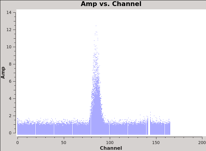
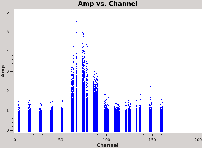
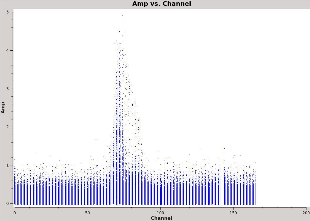
We will make 345 GHz continuum images for the two regions. We use the task tclean over the channels that are free of the line emission; we avoid the edge channels which tend to be noisier due to bandpass rolloff effects. The line-free channels are found by plotting the average spectrum (all fields). We find the CO(3-2) line from channels 50 to 100 in the southern mosaic (Figure 1), and from 70 to 100 in the northern mosaic (Figure 2).
# In CASA
os.system('rm -rf Antennae_North-AMPvsCH.png')
plotms(vis='Antennae_North.cal.ms', xaxis='channel', yaxis='amp',
      avgtime='1e8', avgscan=True, plotfile='Antennae_North-AMPvsCH.png', showgui=True)
# In CASA
os.system('rm -rf Antennae_South-AMPvsCH.png')
plotms(vis='Antennae_South.cal.ms', xaxis='channel', yaxis='amp',
      avgtime='1e8', avgscan=True, plotfile='Antennae_South-AMPvsCH.png', showgui=True)
The avgtime is set to a large value so that it averages over all the integrations, and avgscan is set to allow averaging of the different scans.
Next we create continuum images from the line-free channels.
Northern Continuum Mosaic
For illustrative purposes we first make a dirty image to see if there is emission and what the exact beam size is. It should be on the order of 1" but this will vary a bit according to the uv-coverage in the actual data. We will start with a cell size of 0.2" to oversample the beam by a factor of 5. The imsize needs to be large enough given the cell size to comfortably encompass the mosaic. From the mosaic footprints shown in the Overview, we can see that the Northern mosaic imsize needs to be about 1 arcmin. With 0.2" pixels, this requires imsize=300.
Other essential tclean parameters for this case include:
- vis='Antennae_North.cal.ms' : The calibrated dataset on the science target. tclean will always use the CORRECTED DATA column (if it exists).
- imagename='Antennae_North.Cont.Dirty' : The base name of the output images:
- <imagename>.image # the final restored image
- <imagename>.pb # the primary beam response
- <imagename>.image.pbcor # the primary beam-corrected image (if pbcor=True)
- <imagename>.weight # the primary beam coverage (gridder=’mosaic’ or 'awproject' only)
- <imagename>.model # the model image
- <imagename>.residual # the residual image
- <imagename>.psf # the synthesized (dirty) beam
- spw='0:1~50;120~164' : To specify only the line-free channels of spectral window 0.
- specmode='mfs' : Multi-Frequency Synthesis: The default mode, which produces one image from all the specified data combined. This will grid each channel independently before imaging. For wide bandwidths this will give a far superior result compared to averaging the channels and then imaging.
- restfreq='345.79599GHz' : The rest frequency of CO(3-2) can be found with splatalogue.
- niter=0: Maximum number of tclean iterations. (niter=0 will do no cleaning)
In CASA 5.4 and later, tclean calls with gridder=mosaic have an additional parameter mosweight with a default of True. When mosweight=True, the gridder weights each field in the mosaic independently. The mosweight parameter is particularly important for mosaics with non-uniform sensitivity, with rectangular shapes, or when using more uniform values of robust Briggs weighting.
Starting in CASA 6.2, the beam-fitting algorithm has been updated.
# In CASA
os.system('rm -rf Antennae_North.Cont.Dirty*')
tclean(vis='Antennae_North.cal.ms', imagename='Antennae_North.Cont.Dirty',
      field='', phasecenter=12,
      specmode='mfs',
      deconvolver='hogbom',
      restfreq='345.79599GHz',
      spw='0:1~50;120~164',
      gridder='mosaic', mosweight=True,
      imsize=300, cell='0.2arcsec',
      interactive=False, niter=0)
After tclean has finished, you should now open the image in CARTA. If using NRAO machines, you can open a new terminal tab, cd to the working directory, then type:
# in terminal
carta --no_browser
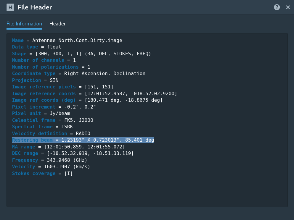
Copy the output URL into a browser to view your CARTA session. Select Antennae_North.Cont.Dirty.image. Before clicking Load, you will see File Information displayed. The restoring beam size is about 1.23" x 0.72", with a position angle (P.A.) of 85.4 degrees. Once you load the image, you can see this information again by opening the Header dialog and selecting the File Information tab (see Fig 3).
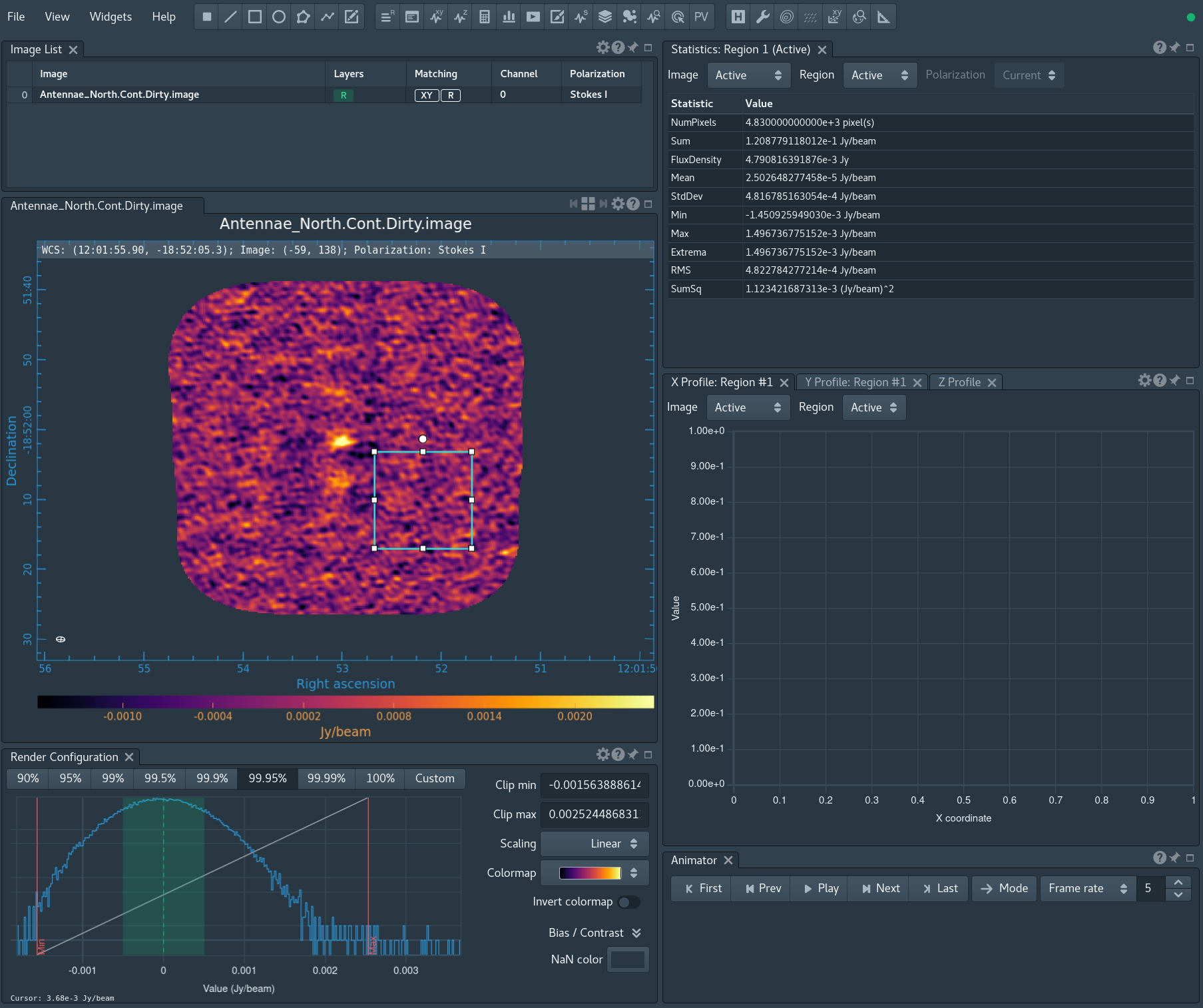
Yes, there is definitely a detection in the vicinity of the Northern nucleus. Draw a region near (but not including) the center and open the Statistics widget. The rms noise is about 0.5 mJy/beam in the dirty image (see Fig 4).
Next we switch to refined values of cell='0.13arcsec' and imsize=500 based on the observed beam size. We also switch to interactive mode so that you can create a clean mask using the polygon tool (note you need to double click inside the polygon region to activate the mask). We have included an example mask to use in Antennae_Band7_CalibratedData.tgz. If you would like to use your own mask, make sure to removed the mask file before running the command below. Otherwise, you can edit the mask within the clean GUI. See TWHydraBand7_Imaging_3.4#Image_and_Self-Calibrate_the_Continuum for a more complete description of interactive clean and mask creation.
- niter=1000: Maximum number of clean iterations -- we will stop interactively
- threshold='0.4mJy' : Stop cleaning if the maximum residual is below this value (the dirty rms noise)
- interactive=True: Clean will be periodically interrupted to show the residual clean image. Interactive clean mask can be made. If no mask is created, no cleaning is done.
# In CASA
for ext in ['.image','.model','.image.pbcor','.psf','.residual','.pb','.sumwt','.weight']:
    rmtables('Antennae_North.Cont.Clean'+ext)

tclean(vis='Antennae_North.cal.ms', imagename='Antennae_North.Cont.Clean',
     field='', phasecenter=12,
     deconvolver='hogbom',
     specmode='mfs', restfreq='345.79599GHz',
     spw='0:1~50;120~164',
     gridder='mosaic', mosweight=True,
     imsize=500, cell='0.13arcsec',
     interactive=True,
     niter=1000, threshold='0.4mJy')
If you get an error using rmtables similar to "Cannot delete file <filename> because table is still open in this process," you may need to close CASA and/or CARTA to unlock the files.
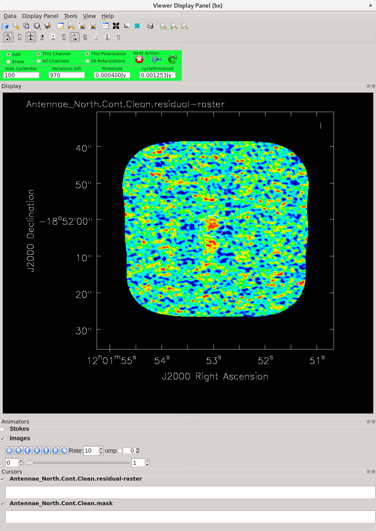
The residuals are "noise-like" after only ~30 iterations (see Figure 5), so hit the red X symbol in the interactive window to stop cleaning here.
Note that if you run the tclean task again with the same imagename, without deleting the existing <imagename>.* files, tclean assumes that you want to continue cleaning the existing images. We put an rm command before the tclean command to guard against this, but sometimes this is what you want.
Southern Continuum Mosaic
For the southern mosaic we modify the phasecenter, mosaic imsize, and the line-free channels (spw) to be consistent for this mosaic. We also bypass the dirty image step we did above for the Northern mosaic. As above, the mosaic size can be judged from the Overview. We expect the beam to be about the same and use the same cell size. Again, you can use the provided mask or make your own.
# In CASA
for ext in ['.image','.model','.image.pbcor','.psf','.residual','.pb','.sumwt','.weight']:
    rmtables('Antennae_South.Cont.Clean'+ext)

tclean(vis='Antennae_South.cal.ms', imagename='Antennae_South.Cont.Clean',
      field='', phasecenter=15,
      specmode='mfs', restfreq='345.79599GHz',
      spw='0:1~30;120~164',
      gridder='mosaic', mosweight=True, deconvolver='hogbom',
      imsize=750, cell='0.13arcsec',
      interactive=True,
      niter=1000, threshold='0.4mJy')
The beam size is reported in the logger as 1.14"x0.66" with P.A.=61.5 deg, which is a little better than the North beam due to better uv-coverage.
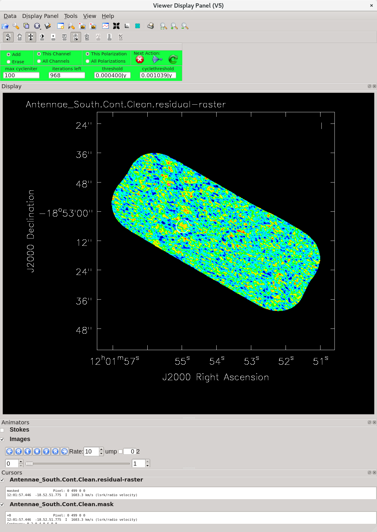
Click the green arrow to run one major cycle. We hit the stopping threshold after ~32 iterations (minor cycles). The residuals now look noise-like and we can stop cleaning (see Figure 6). Hit the red X to close the tclean GUI.
Image Statistics
You can determine statistics for the images using the task imstat:
# In CASA
imstat('Antennae_North.Cont.Clean.image')
imstat('Antennae_South.Cont.Clean.image')
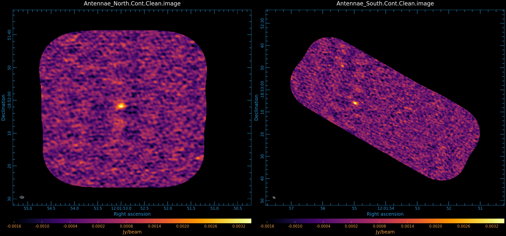
From this we find that for the Northern continuum image the peak (max) is 3.82 mJy/beam and the rms (sigma) is 0.49 mJy/beam. For the Southern continuum we find a peak (max) of 4.77 mJy/beam and an rms (sigma) of 0.47 mJy/beam.
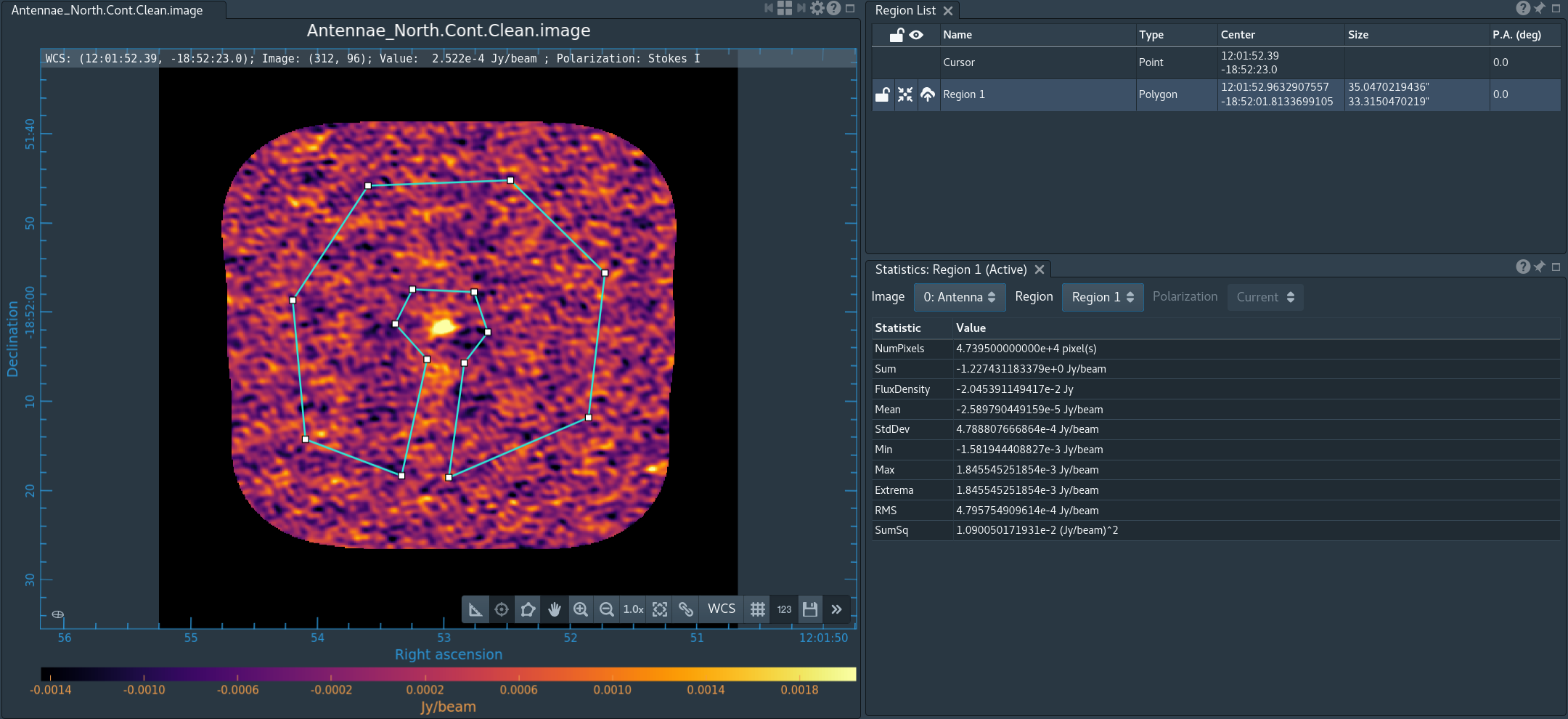
However, the calculation of the rms comes with a couple of caveats. First, the mosaic primary beam response rolls off toward the edges of the mosaic, as do correspondingly the flux density and rms. Thus if you don't restrict the measurement to areas of full sensitivity, the apparent rms is skewed downward. Second, since there is real emission in the image, the rms will be skewed upward (with the error increasing with brighter emission). Both can be solved by picking boxes that exclude the edges of the mosaic and the real emission. It is often easier to use CARTA to display the image and then interactively use the region tools to get the statistics.
Open 'Antennae_North.Cont.Clean.image' in CARTA. Draw a region that avoids the edges and emission (see Figure 5), and view the Statistics widget. You may measure an rms that differs by a few percent from the value reported by imstat. Repeat this for 'Antennae_South.Cont.Clean.image'. Again, you may measure an rms slightly different than what we got from using imstat with no constraints.
How does this compare to theory? You can find out using the ALMA sensitivity calculator. The continuum bandwidth of the Northern mosaic is about 1 GHz and about 0.85 GHz for the Southern mosaic. The number of antennas is about 12 and the time on a single pointing is about 300s. This yields an expected rms of about 1 mJy/beam. However, this needs to be decreased by about a factor of 2.5 near the center of the mosaic due to the hexagonal Nyquist sampling of the mosaic (radial spacing~0.37*HPBW) for a theoretical rms of about 0.4 mJy/beam, in good agreement with observation.
Finally, use CARTA to export .png images of both the North and South mosaics. You can view the images side by side by enabling multi-panel view in the image viewer, and you may wish to enable "Raster scaling matching."
Continuum subtraction
In these data, the continuum emission is too weak to contaminate the line emission (i.e. the peak continuum emission is less than the rms noise in the spectral line channels). Nevertheless, for illustrative purposes we demonstrate how to subtract the continuum emission in the uv-domain using the task uvcontsub.
# In CASA
uvcontsub(vis='Antennae_North.cal.ms', outputvis='Antennae_North.cal.ms.contsub', fitspec='0:1~50;120~164', fitorder=1)
# In CASA
uvcontsub(vis='Antennae_South.cal.ms', outputvis='Antennae_South.cal.ms.contsub', fitspec='0:1~30;120~164', fitorder=1)
Here, fitspec specifies the line-free channels to fit. Higher fit order than 1 are not recommended. If you do not have line-free channels on both sides of the line fitorder=0 is recommended.
CO(3-2) Imaging
Choose Frame and Velocity Channels
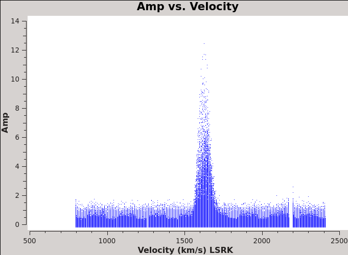
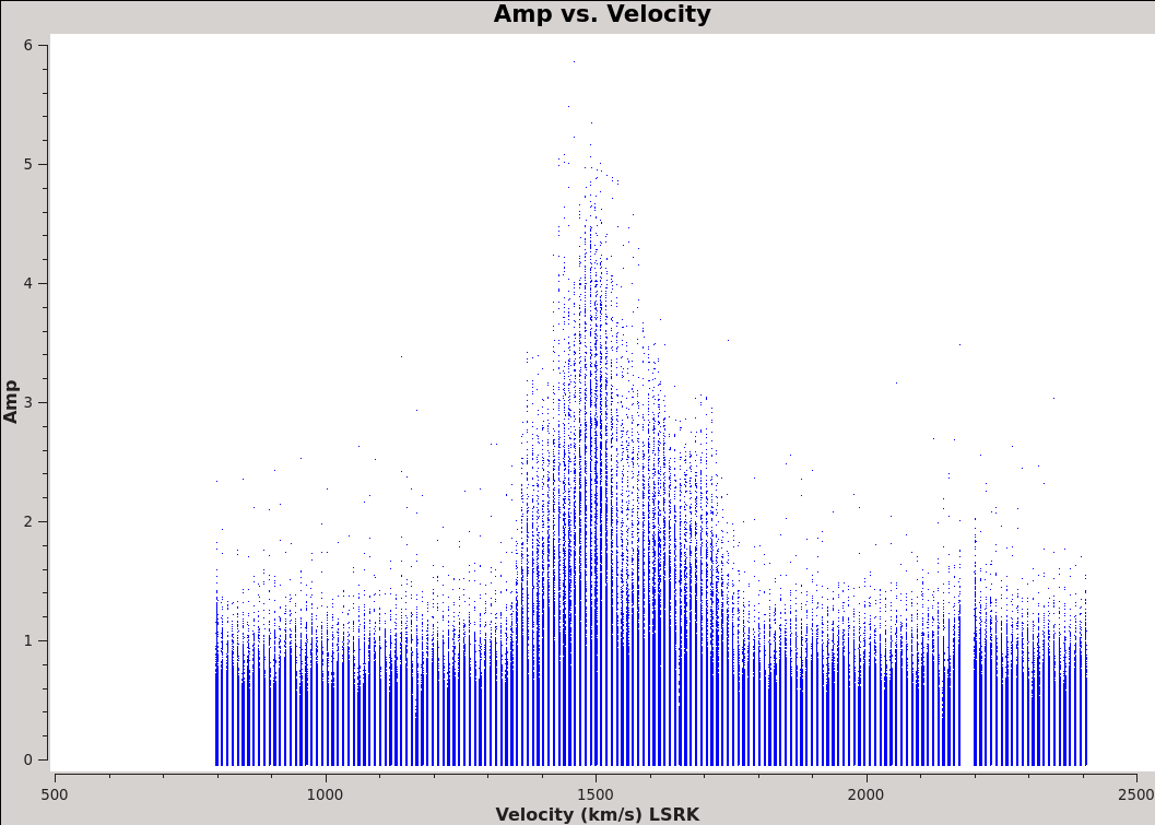
Now we are ready to make cubes of the line emission. The imaging parameters are similar to the continuum except for those dealing with the spectral setup: specmode, start, width, nchan, restfreq, and outframe parameters. As noted above, setting specmode='mfs' gives an output image with only one channel, and is used for continuum imaging. specmode='cube' creates output data cubes with one or more channels.
Data are taken using constant frequency channels. For spectral line analysis it's often more useful to have constant velocity channels, and this is also the best way to make images of multiple lines with the exact same channelization for later comparison. For specmode='cube', the desired start and width also need to be given in velocity units for the desired output frame.
It is important to note that ALMA does not do on-line Doppler Tracking and the native frame of the data is TOPO. If you do not specify outframe the output cube will also be in TOPO, which is not very useful for scientific analysis. The Doppler Shift is taken out during the regridding to the desired outframe in tclean or alternatively it can be done separately by the cvel task which would need to be run before tclean.
To see what velocity parameters you want to set in tclean, it is useful to make a plot in plotms in the desired output frame. Note these plots take a little longer because of the frame shift. In order to compare with recent SMA data, we chose LSRK, but it should be noted that many papers of this source are in the BARY frame.
# In CASA
os.system('rm -rf North_CO3_2_vel.png')
plotms(vis='Antennae_North.cal.ms.contsub', xaxis='velocity', yaxis='amp',
       avgtime='1e8', avgscan=True, transform=True, freqframe='LSRK',
       restfreq='345.79599GHz', plotfile='North_CO3_2_vel.png', showgui=True)
# In CASA
os.system('rm -rf South_CO3_2_vel.png')
plotms(vis='Antennae_South.cal.ms.contsub', xaxis='velocity', yaxis='amp',
      avgtime='1e8', avgscan=True, transform=True, freqframe='LSRK',
      restfreq='345.79599GHz', plotfile='South_CO3_2_vel.png', showgui=True)
Northern Mosaic Cube
Similar to continuum, it is very important that you make a clean mask. For this example we will create a single clean mask that encompasses the line emission in every channel and apply it to all channels. This is much better than no clean mask, though not quite as good as making an individual mask for each channel.
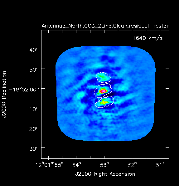
Notable parameters included in the tclean call are:
- specmode='cube', outframe='LSRK', restfreq='345.79599GHz'. We use 'cube' mode to create an output data cube. We set the velocity information in the Local Standard of Rest frame (kinematic definition), and use the rest frequency of the CO(3-2) line.
- nchan=70, start='1200km/s', width='10km/s': To produce a data cube with 70 channels, starting at 1200 km/s, and with velocity widths of 10 km/s. That will include all the CO(3-2) emission in both mosaics.
- imsize=500, cell='0.13arcsec': An image size of 65 arcsec, with pixels of 0.13 arcsec (about one-fifth the minor axis of the synthesized beam). We make the imsize larger than the mosaic to increase the dirty beam image size, as the emission is quite extended along the mosaic.
- weighting='briggsbwtaper', robust=0.5: Weighting to apply to visibilities. Weighting has been changed to 'briggsbwtaper'. This is a new weighting scheme available starting in CASA 6.2. See Imaging Algorithms for more information. We use robustness parameter 0.5 (in between natural and uniform weighting).
- niter=20000: Maximum number of clean iterations. With complex emission structure like that found in the Antennae CO data, we will need a large number of iterations to clean the emission. Note that you can increase the number of iterations allowed on-the-fly in the interactive tclean window.
- threshold='5.0mJy': Stop cleaning if the maximum residual is below this value.
The threshold is set to roughly the rms of a single line-free channel for each dataset.
- savemodel='modelcolumn': This saves the clean model to the ms file. We will need this for self-calibration later.
# In CASA
for ext in ['.image','.model','.image.pbcor','.psf','.residual','.pb','.sumwt','.weight']:
    rmtables('Antennae_North.CO3_2Line.Clean'+ext)

tclean(vis='Antennae_North.cal.ms.contsub',
      imagename='Antennae_North.CO3_2Line.Clean',
      spw='0', field='', phasecenter=12,
      specmode='cube', outframe='LSRK', restfreq='345.79599GHz',
      nchan=70, start='1200km/s', width='10km/s',
      gridder='mosaic', mosweight=True,
      deconvolver='hogbom',
      imsize=500, cell='0.13arcsec', pblimit=0.2,
      restoringbeam='common',
      interactive=True,
      weighting='briggsbwtaper', robust=0.5,
      niter=20000, threshold='5.0mJy',
      savemodel='modelcolumn')
Figure 10 shows what the final clean box should look like. Cycle through the channels until you reach ~1650 km/s, where you can more easily see where to draw the clean box around the CO emission. Be sure to check the circle next to 'All Channels' when making your clean mask. Now clean using the green circle arrow. You can watch the progress in the logger. When the first ~650 iterations are done, the viewer will show the residual map for each channel. Cycle through the channels and see whether you are still happy with the clean box in each channel with significant signal. The "Erase" button can help you fix mistakes. If necessary, adjust. It is often useful to adjust the colorscale with the "plus" (crossing arrows) icon. To make it go a bit faster, you can increase iteration interactively to 200 or 300, but don't overdo it.
These data are pretty severely dynamic range limited, in part due to the sparse uv coverage. In other words, the noise in bright channels is set by a maximum signal-to-noise. This effectively prevents us from stopping clean based on an rms based threshold because the effective rms changes as a function of the brightest signal in each channel. Thus, in this case we need to stop clean interactively. Below an approximate number of iterations is given to help you decide when to quit. The threshold that is set in the CO(3-2) clean commands are about equal to the noise in a line-free channel and is only there to prevent clean running forever if you fail to stop it. You are not intended to clean to this threshold.
Also, we are going to self-calibrate the data so it's best to be conservative here - it can be difficult in images like these to discern real features from artifacts. If in doubt, don't include it in the clean mask. Keep cleaning and see if the feature becomes weaker. You cannot lose real emission by not masking it, but you can create a brighter feature by masking an artifact.
Stop cleaning after about ~7000 iterations (Red X), when the artifacts start to look as bright as the residual. Note again that we are not cleaning to the theoretical noise level.
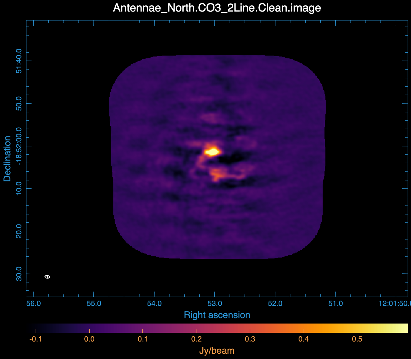
Inspect the resulting data cube in CARTA (Fig 11):
Antennae_North.CO3_2Line.Clean.image
Southern Mosaic Cube
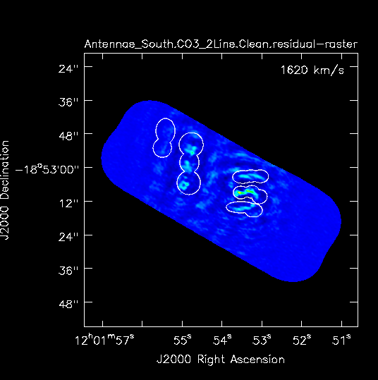
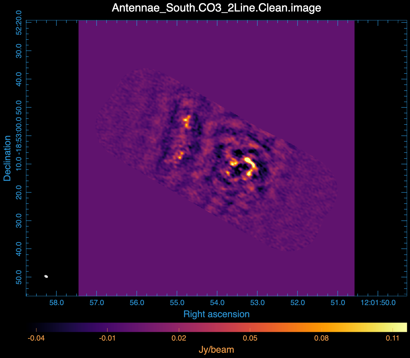
Repeat the process for Southern mosaic.
# In CASA
for ext in ['.image','.model','.image.pbcor','.psf','.residual','.pb','.sumwt','.weight']:
    rmtables('Antennae_South.CO3_2Line.Clean'+ext)

tclean(vis='Antennae_South.cal.ms.contsub',
      imagename='Antennae_South.CO3_2Line.Clean',
      spw='0', field='', phasecenter=15,
      specmode='cube', outframe='LSRK', restfreq='345.79599GHz',
      nchan=70, start='1200km/s', width='10km/s',
      gridder='mosaic', deconvolver='hogbom',
      imsize=750, cell='0.13arcsec', pblimit=0.2,
      restoringbeam='common',
      interactive=True,
      weighting='briggsbwtaper', robust=0.5,
      niter=20000, threshold='5.0mJy',
      savemodel='modelcolumn')
Clean about 8,000 iterations before stopping. Inspect the resulting data cube in CARTA (Fig 13):
Antennae_South.CO3_2Line.Clean.image
Statistics
For each mosaic, in CARTA, draw regions in both a line-free channel and the channel with the strongest emission, and evaluate using the Statistics widget.
The line-free channel rms for the northern and southern mosaics are about 4.0 mJy/beam and 3.5 mJy/beam, respectively. However, in a bright channel, this degrades to about 18 mJy/beam and 9 mJy/beam, respectively. This is the aforementioned dynamic range limit.
Using the ALMA sensitivity calculator, a bandwidth of 10 km/s, dual polarization, 12 antennas, and the time on a single pointing of about 300s yields an rms of about 9.0 mJy/beam. As described above, the Nyquist sampled hexagonal mosaic improves this by a factor of about 2.5, for an expected rms noise of about 3.6 mJy. In line-free channels, our image is close to this theoretical rms.
Self Calibration
Next we attempt to self-calibrate the uv-data. The process of self-calibration tries to adjust the data to better match the model image that you give it. When tclean is run, it saves a uv-model of the resulting image in the MODEL column of the measurement set if savemodel='modelcolumn'. This model can be used to self-calibrate the data using gaincal. That is why it is important to make the model as good as you can by making clean masks.
Mosaics can be tricky to self-calibrate. The reason is that typically only a few of the pointings may have strong emission. The stronger the signal, the stronger the signal-to-noise will be for a given self-calibration solution interval (solint). This means that typically only a few fields are strong enough for self-calibration, though it can still bring about overall improvement to apply these solutions to all fields. The fine tuning of each field in the mosaic over small solutions intervals is often impossible. Indeed fine-tuning only a few fields in the mosaic on small time scales can result in a mosaic with dramatically different noise levels as a function of position. Below, we will simply attempt to self-calibrate on the strongest field in the mosaic, obtaining one average solution per original input dataset.
Here, the continuum is far too weak so we will use the CO(3-2) line emission. To increase signal-to-noise it is often helpful to limit solutions to the range of channels containing the strongest line emission.
We will also use gaintype='T' to tell CASA to average the polarizations before deriving solutions which gains us a sqrt(2) in sensitivity.
Northern Mosaic Selfcal
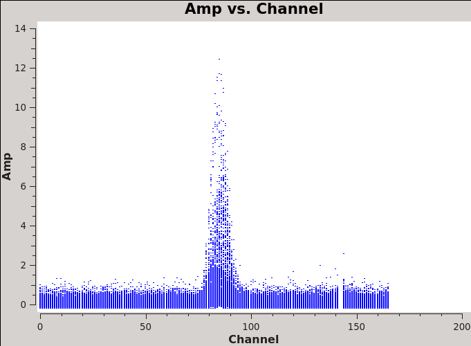
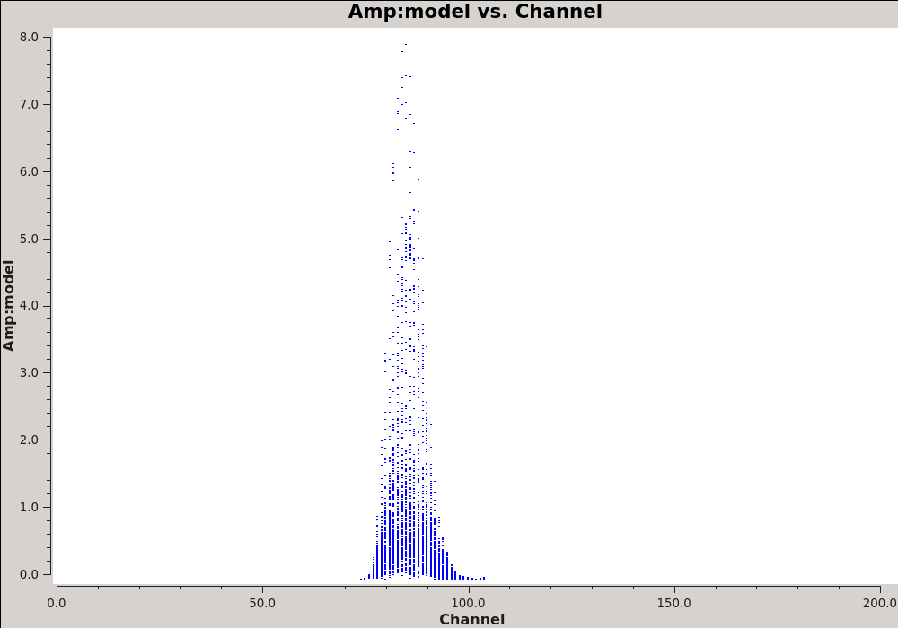
The strongest emission in the Northern mosaic comes from the center pointing, already identified above as field='12'. Below we make a uv-plot of the spectral line emission from this field to choose only the strongest channels to include in the self-calibration. It is essential that the self-calibration channel range be chosen based on the UV data and not on the image cube. This is because the channels in the image cube were modified by the velocity/channel specifications in the first invocation of clean. This plot shows the channel range of the uv data.
# In CASA
plotms(vis='Antennae_North.cal.ms.contsub', spw='', xaxis='channel', yaxis='amp', field='12',
       avgtime='1e8', avgscan=True, ydatacolumn='data', plotfile='North_selfchan_data.png',
       height=800, width=1000, overwrite=True, showgui=True)
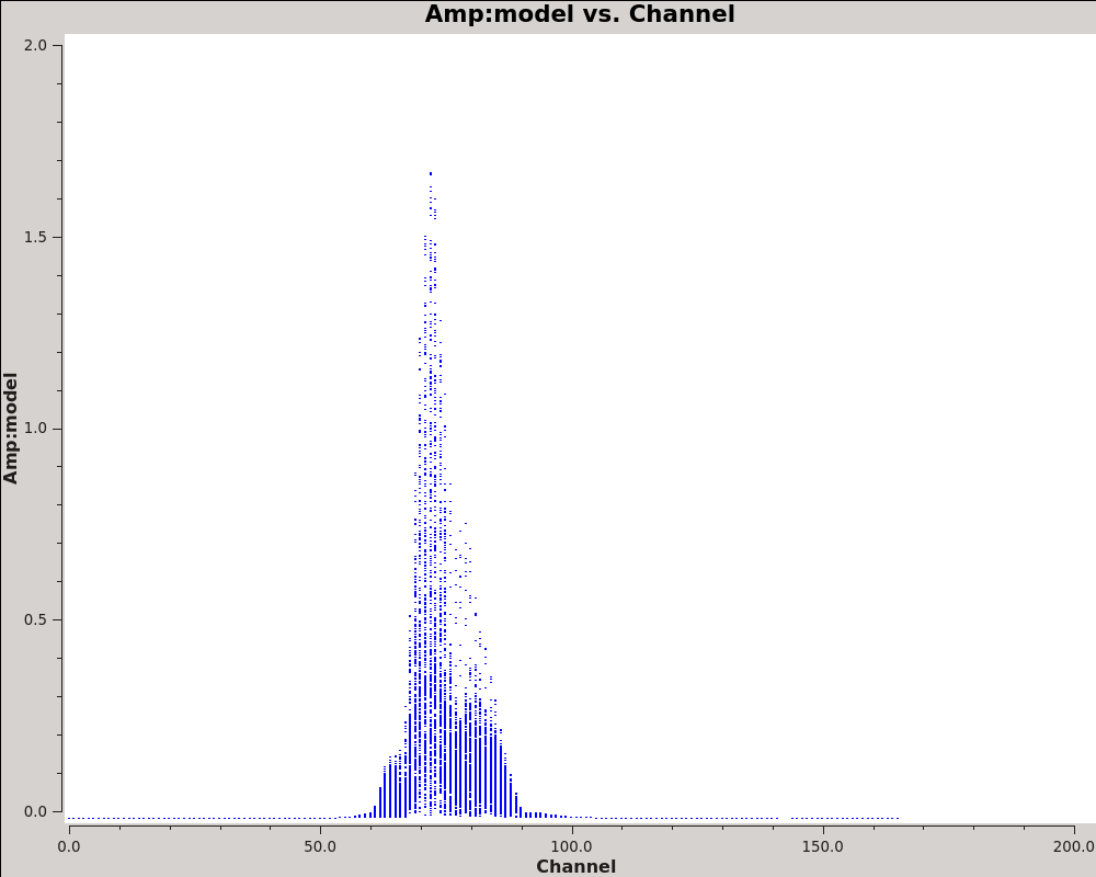
We also want to check the channel amplitudes in the model column of the measurement set. The depth of the initial clean will determine what model channels have emission. (A very shallow clean could potentially produce a model with emission over a small range of channels.) Self calibration will attempt to make the data look like the model. Therefore, it is important that we select a channel range where the model is realistic.
# In CASA
plotms(vis='Antennae_North.cal.ms.contsub', spw='', xaxis='channel', yaxis='amp', field='12',
       avgtime='1e8', avgscan=True, ydatacolumn='model', plotfile='North_selfchan_model.png',
       height=800, width=1000, overwrite=True, showgui=True)
While the model looks reasonable across the channels where we imaged the data, the model amplitudes are set to 0 elsewhere by default. We will perform self-calibration only on the channels we imaged in the first cube, with significant signal in the line emission.
Next, we remind ourselves of the timing of the various observations. Examine the listobs output, Antennae_North.cal.listobs.txt. Each dataset has 2 or 3 observations of field 12. Each time, it's observed for about 25 seconds. We set solint='3600s' to get one solution per dataset.
# In CASA
gaincal(vis='Antennae_North.cal.ms.contsub', caltable='north_self_1.pcal',
        solint='3600s', combine='scan', gaintype='T', field='12',
        refant='DV09', spw='0:82~89', minblperant=4,
        calmode='p', minsnr=2)
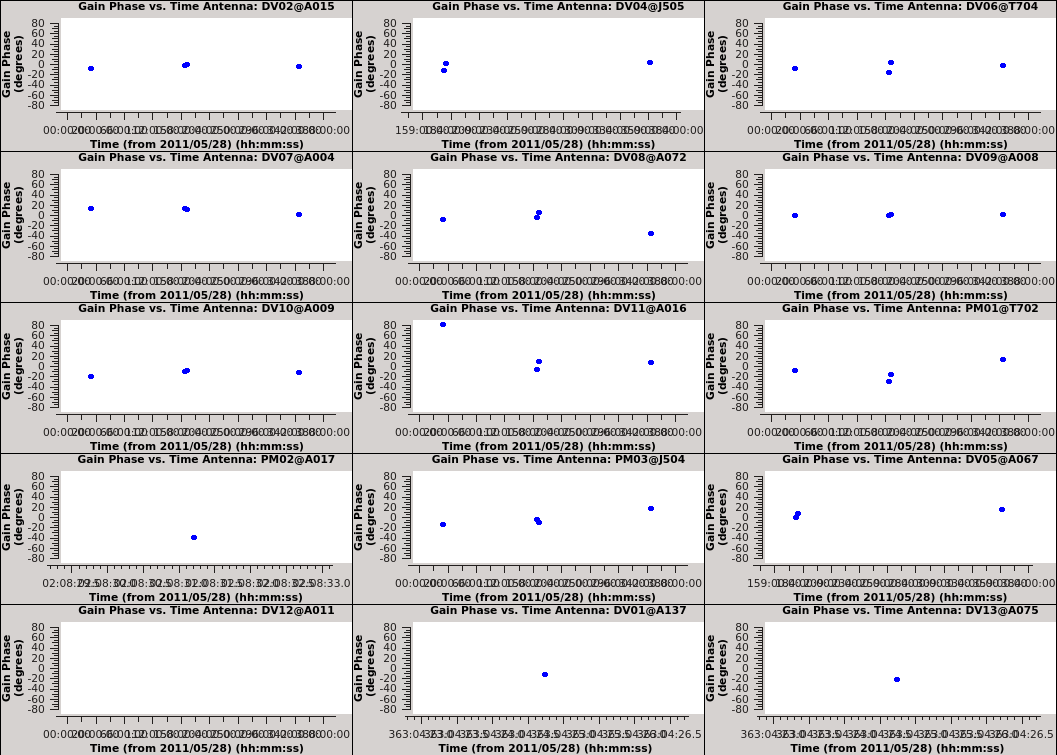
Plot the calibration solutions. Note that when iteraxis is set, plotms appends the axes being iterated over to the output filename specified in plotfile; this can make for rather unwieldy filenames but is useful for ALMA pipeline purposes.
# In CASA
plotms(vis='north_self_1.pcal', xaxis='time', yaxis='phase',
        spw='', field='', antenna='',
        iteraxis='antenna', gridrows=5, gridcols=3, plotrange=[0,0,-80,80],
        plotfile='north_pcal1_phase.png', showgui=True)
Apply the solutions to all fields and channels with applycal, which will overwrite the corrected data column:
# In CASA
applycal(vis='Antennae_North.cal.ms.contsub', field='',
        gaintable=['north_self_1.pcal'], calwt=False)
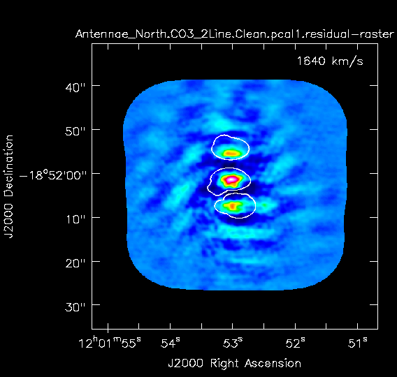
Re-image the data with the selfcal applied. Remember that tclean always uses the corrected data column if it exists. We will start with the same mask that we ended with before.
# In CASA
os.system('rm -rf Antennae_North.CO3_2Line.Clean.pcal1*')
tclean(vis='Antennae_North.cal.ms.contsub',
      imagename='Antennae_North.CO3_2Line.Clean.pcal1',
      spw='0', field='', phasecenter=12,
      specmode='cube', outframe='LSRK', restfreq='345.79599GHz',
      nchan=50, start='1300km/s', width='10km/s',
      gridder='mosaic', mosweight=True,
      deconvolver='hogbom',
      imsize=500, cell='0.13arcsec', pblimit=0.2,
      restoringbeam='common',
      interactive=True, mask='Antennae_North.CO3_2Line.Clean.mask',
      weighting='briggsbwtaper', robust=0.5,
      niter=20000, threshold='5.0mJy',
      savemodel='modelcolumn')
After 1000-2000 iterations or so, inspect each channel to see if there is more emission that needs to be included in the mask. Remember to select the "all channels" toggle. Stop after 5000 or so iterations.
Compare the original and self-calibrated images in CARTA to determine if there has been improvement:
Antennae_North.CO3_2Line.Clean.image
Antennae_North.CO3_2Line.Clean.pcal1.image
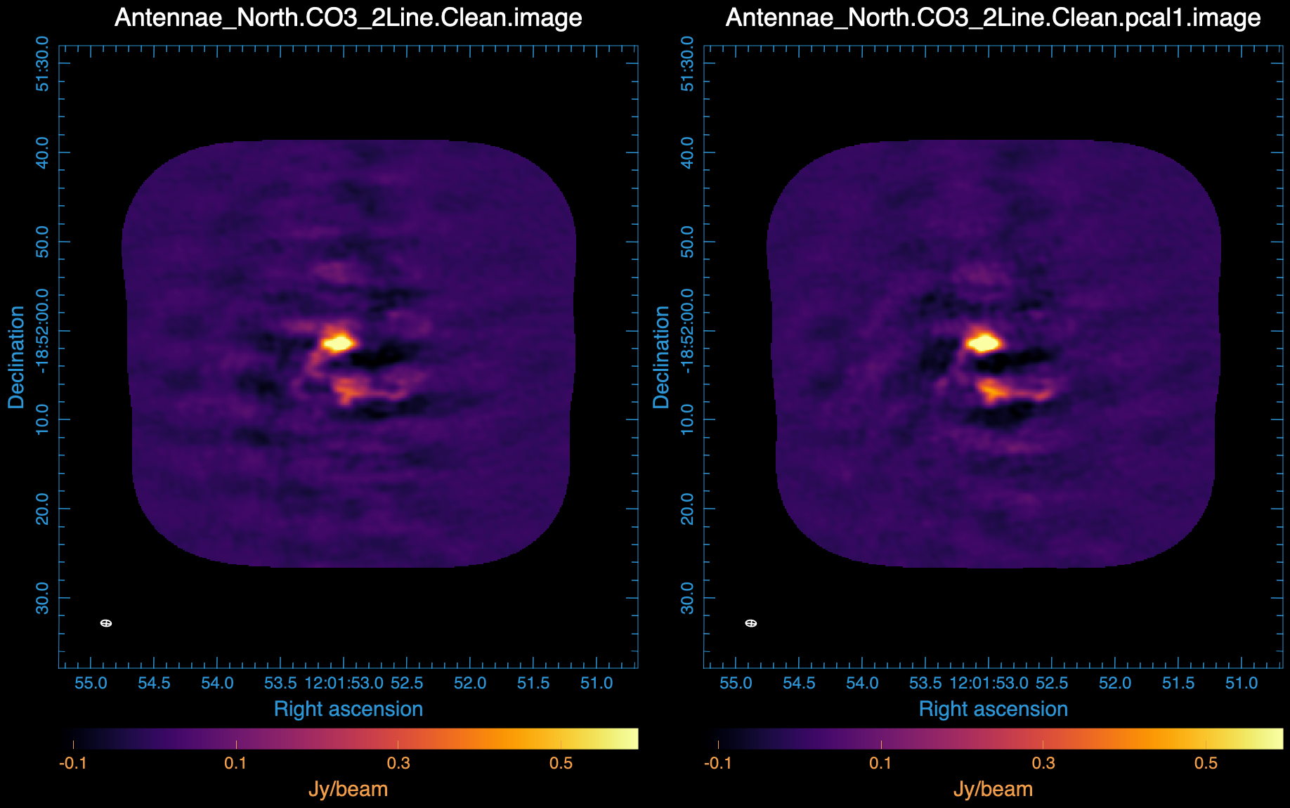
The images may look quite similar at first. Examining the image statistics, the peak flux density should have increased substantially while the rms noise is about the same. This is reasonable for this self-calibration case because we have mostly adjusted relative position offsets between the datasets and not taken out any short-term phase variations which would reduce the rms.
Note that attempts to push the selfcal to shorter solint (for example to each scan of field=12) did not yield additional improvement.
If you used standard='Butler-JPL-Horizons 2012' when running setjy during the calibration process, you may see an increase of approximately 20% in the peak flux density of bright channels.
Southern Mosaic Selfcal
Now repeat the self-calibration process for the Southern mosaic. It is a bit tougher in this case to pick the best field. The most compact bright emission is toward Field 11 in the Overview. Adjusting for the renumbering of Field IDs after the final calibration split, this becomes Field 7.
From the plots of data and model amplitude, we can assess the brightest channels to selfcal and image:
# In CASA
plotms(vis='Antennae_South.cal.ms.contsub', spw='', xaxis='channel', yaxis='amp',
       field='7', avgtime='1e8', avgscan=True, ydatacolumn='data',
       plotfile='South_selfchan_data.png', height=800, width=1000, overwrite=True, showgui=True)
# In CASA
plotms(vis='Antennae_South.cal.ms.contsub', spw='', xaxis='channel', yaxis='amp',
       field='7', avgtime='1e8', avgscan=True, ydatacolumn='model',
       plotfile='South_selfchan_model.png', height=800, width=1000, overwrite=True, showgui=True)
Examine the listobs output, Antennae_South.cal.listobs.txt. The timing in the 6 Southern datasets is similar to the North, with each lasting about 1 hour.
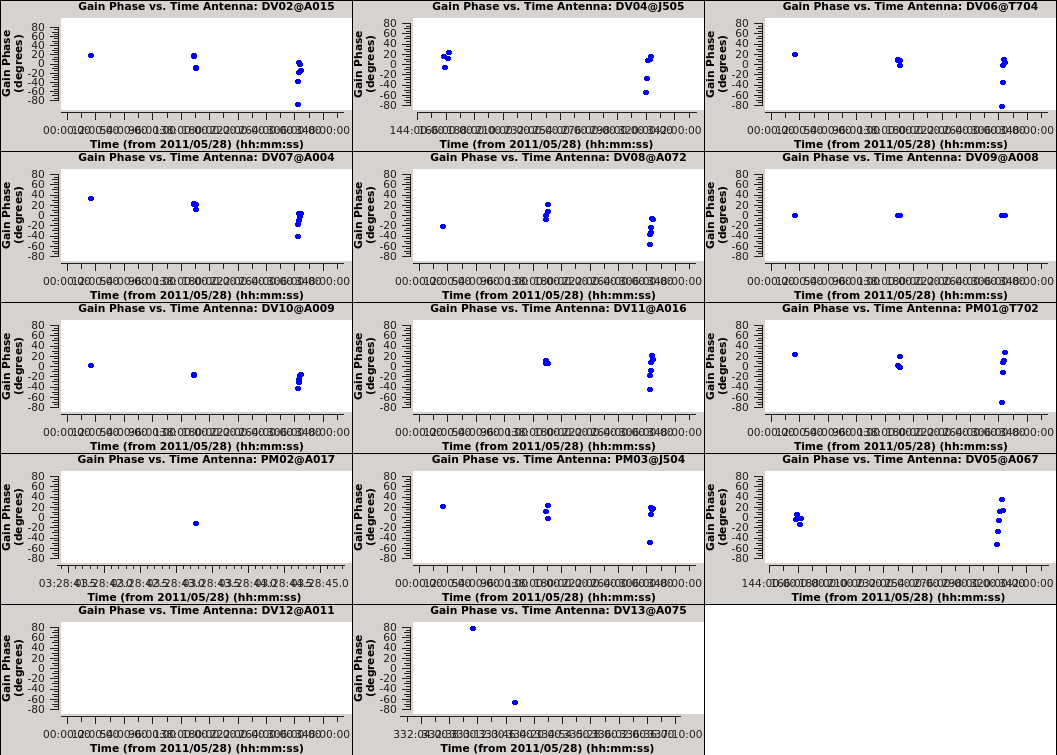
Solve for the self-calibration phase corrections:
# In CASA
gaincal(vis='Antennae_South.cal.ms.contsub', caltable='south_self_1.pcal',
        solint='3600s', combine='scan', gaintype='T', field='7',
        refant='DV09', spw='0:70~85', minblperant=4,
        calmode='p', minsnr=2)
Plot the selfcal solutions:
# In CASA
plotms(vis='south_self_1.pcal', xaxis='time', yaxis='phase',
        spw='', field='', antenna='',
        iteraxis='antenna', gridrows=5, gridcols=3, plotrange=[0,0,-80,80],
        plotfile='south_pcal1_phase.png', showgui=True)
Apply the solutions:
# In CASA
applycal(vis='Antennae_South.cal.ms.contsub', field='',
        gaintable=['south_self_1.pcal'], calwt=False)
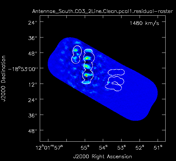
Clean a new cube using the newly corrected data. We will start with the South mosaic mask from before selfcal, and don't forget to select All Channels if modifying the mask:
# In CASA
os.system('rm -rf Antennae_South.CO3_2Line.Clean.pcal1*')

tclean(vis='Antennae_South.cal.ms.contsub',
      imagename='Antennae_South.CO3_2Line.Clean.pcal1',
      spw='0', field='', phasecenter=15,
      specmode='cube', outframe='LSRK', restfreq='345.79599GHz',
      nchan=50, start='1300km/s', width='10km/s',
      gridder='mosaic', mosweight=True, deconvolver='hogbom',
      imsize=750, cell='0.13arcsec', pblimit=0.2,
      restoringbeam='common',
      interactive=True, mask='Antennae_South.CO3_2Line.Clean.mask',
      weighting='briggsbwtaper', robust=0.5,
      niter=40000, threshold='5.0mJy',
      savemodel='modelcolumn')
After 4000 iterations or so, inspect each channel to see if there is more emission that needs to be included in the mask. Stop after 20000 or so iterations.
Compare the before and after selfcal images in CARTA, and examine the rms and peak flux density of a couple bright channels:
Antennae_South.CO3_2Line.Clean.image
Antennae_South.CO3_2Line.Clean.pcal1.image
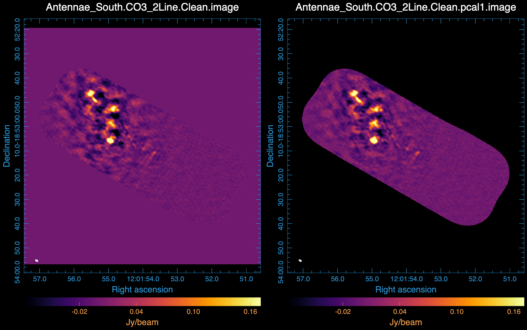
Image Analysis
Moment Maps
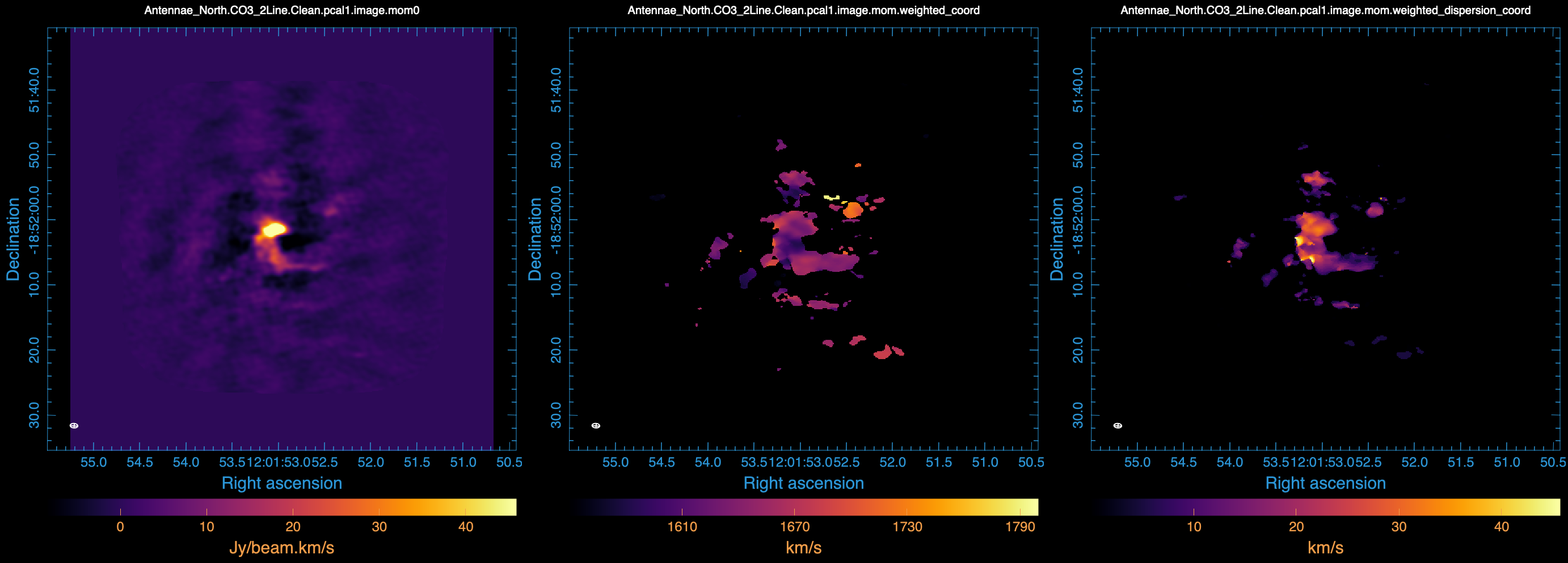
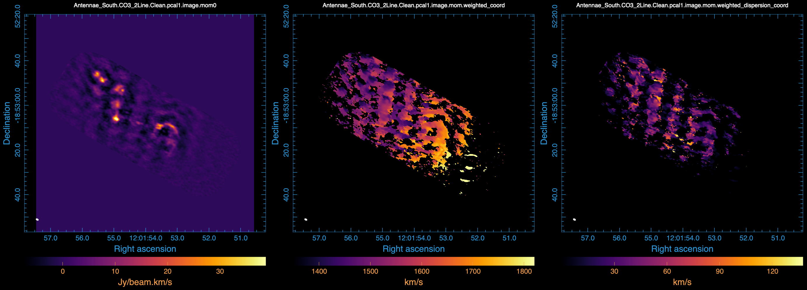
Next we will make moment maps for the CO(3-2) emission.
Moment 0 = integrated intensity
Moment 1 = intensity weighted velocity field
Moment 2 = intensity weighted velocity dispersion
Above we determined the rms noise levels for both the North and South mosaics in both a line-free and a line-bright channel. We want to limit the channel range of the moment calculations to those channels with significant emission. One good way to do this is to open the cube in CARTA overlaid with 3-sigma contours, with sigma corresponding to the line-free rms (North ~ 4.0 mJy/beam, South ~ 3.5 mJy/beam). For North, we find a channel range for significant emission of 21~49. For South, we find a channel range for significant emission of 2~49.
For moment 0 (integrated intensity) maps you do not typically want to set a flux threshold because this will tend to noise bias your integrated intensity.
# In CASA
immoments('Antennae_North.CO3_2Line.Clean.pcal1.image',
          moments=[0], chans='21~49',
          outfile='Antennae_North.CO3_2Line.Clean.pcal1.image.mom0')
# In CASA
immoments('Antennae_South.CO3_2Line.Clean.pcal1.image',
          moments=[0], chans='2~49',
          outfile='Antennae_South.CO3_2Line.Clean.pcal1.image.mom0')
For higher order moments it is very important to set a conservative flux threshold. Typically something like 3sigma, using sigma from a bright line channel works well (North ~ 14 mJy/beam, South ~ 4 mJy/beam). We do this with the mask parameter in the commands below. When making multiple moments, immoments appends the appropriate file name suffix to the value of outfile.
# In CASA
immoments('Antennae_North.CO3_2Line.Clean.pcal1.image',
          moments=[1,2], chans='21~49',
          mask='Antennae_North.CO3_2Line.Clean.pcal1.image>0.014*3',
          outfile='Antennae_North.CO3_2Line.Clean.pcal1.image.mom')
# In CASA
immoments('Antennae_South.CO3_2Line.Clean.pcal1.image',
          moments=[1,2], chans='2~49',
          mask='Antennae_South.CO3_2Line.Clean.pcal1.image>0.004*3',
          outfile='Antennae_South.CO3_2Line.Clean.pcal1.image.mom')
Open your six moment maps in CARTA and export to .png (Figures 22 and 23):
Antennae_North.CO3_2Line.Clean.pcal1.image.mom0
Antennae_North.CO3_2Line.Clean.pcal1.image.mom.weighted_coord
Antennae_North.CO3_2Line.Clean.pcal1.image.mom.weighted_dispersion_coord
Antennae_South.CO3_2Line.Clean.pcal1.image.mom0
Antennae_South.CO3_2Line.Clean.pcal1.image.mom.weighted_coord
Antennae_South.CO3_2Line.Clean.pcal1.image.mom.weighted_dispersion_coord
Exporting Images to Fits
If you want to analyze the data using another software package it is easy to convert from CASA format to FITS.
# In CASA
exportfits(imagename='Antennae_North.Cont.Clean.image',
     fitsimage='Antennae_North.Cont.Clean.image.fits', overwrite=True)
exportfits(imagename='Antennae_North.CO3_2Line.Clean.pcal1.image',
     fitsimage='Antennae_North.CO3_2Line.Clean.pcal1.image.fits', overwrite=True)
exportfits(imagename='Antennae_North.CO3_2Line.Clean.pcal1.image.mom0',
     fitsimage='Antennae_North.CO3_2Line.Clean.pcal1.image.mom0.fits', overwrite=True)
exportfits(imagename='Antennae_North.CO3_2Line.Clean.pcal1.image.mom.weighted_coord',
     fitsimage='Antennae_North.CO3_2Line.Clean.pcal1.image.mom.weighted_coord.fits', overwrite=True)
exportfits(imagename='Antennae_North.CO3_2Line.Clean.pcal1.image.mom.weighted_dispersion_coord',
     fitsimage='Antennae_North.CO3_2Line.Clean.pcal1.image.mom.weighted_dispersion_coord.fits', overwrite=True)
# In CASA
exportfits(imagename='Antennae_South.Cont.Clean.image',
     fitsimage='Antennae_South.Cont.Clean.image.fits', overwrite=True)
exportfits(imagename='Antennae_South.CO3_2Line.Clean.pcal1.image',
     fitsimage='Antennae_South.CO3_2Line.Clean.pcal1.image.fits', overwrite=True)
exportfits(imagename='Antennae_South.CO3_2Line.Clean.pcal1.image.mom0',
     fitsimage='Antennae_South.CO3_2Line.Clean.pcal1.image.mom0.fits', overwrite=True)
exportfits(imagename='Antennae_South.CO3_2Line.Clean.pcal1.image.mom.weighted_coord',
     fitsimage='Antennae_South.CO3_2Line.Clean.pcal1.image.mom.weighted_coord.fits', overwrite=True)
exportfits(imagename='Antennae_South.CO3_2Line.Clean.pcal1.image.mom.weighted_dispersion_coord',
     fitsimage='Antennae_South.CO3_2Line.Clean.pcal1.image.mom.weighted_dispersion_coord.fits', overwrite=True)
Although "FITS format" is supposed to be a standard, in fact most packages expect slightly different things from a FITS image. If you are having difficulty, try setting velocity=True and/or dropstokes=True.
Comparison with previous SMA CO(3-2) data
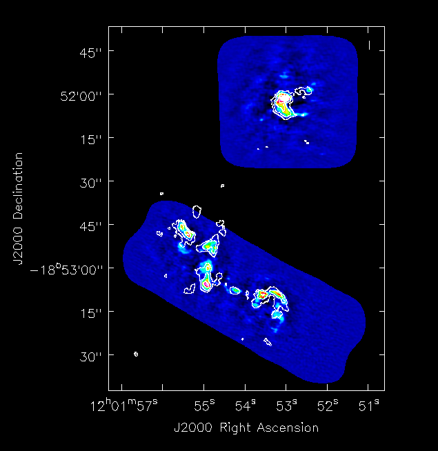
We compare with SMA CO(3-2) data (Ueda, Iono, Petitpas et al. 2012, ApJ, 745, 65). Figure 28 shows a comparison plot between the moment 0 maps of ALMA and SMA data using the viewer. The fluxes, peak locations, and large scale structure are consistent. Both southern and northern components have been combined.
Last checked on CASA Version 6.5.4