First Look at Self Calibration CASA 6
This guide is written for CASA 6.2.1.7 and uses Python 3.
This script steps you through continuum imaging and self calibration of the science data for our science target, TW Hydra.
You should have downloaded the data package as part of the previous imaging tutorial. If you haven't done that yet, check the First Look At Imaging Guide for instructions.
In that first tutorial you made a first continuum image in the previous imaging lesson. We start here by repeating that step and then we iteratively self-calibrate the data, focusing on short-timescale phase corrections.
First, copy the calibrated and flagged data from the working directory. Remember that this is our best version of the data.
# In CASA
os.system("rm -rf sis14_twhya_calibrated_flagged.ms")
os.system("tar -xvf ../working/sis14_twhya_calibrated_flagged.ms.tar")
Run a quick listobs to get oriented:
# In CASA
listobs("sis14_twhya_calibrated_flagged.ms")
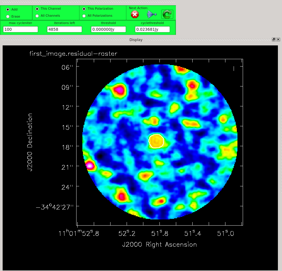
Now, use tclean to make a continuum image of TW Hydra (field 5). This call is interactive, but the automated approach that we used in the last lesson would also work. See the last lesson for details. Remember that the spectral window that we will image here as continuum also contains a N2H+ emission line. In this case, the N2H+ emission is faint enough that neglecting to flag the line channels before imaging makes no difference to the final continuum image. For this and the other continuum first look tutorials, we have thus ignored the line to focus on the basic steps of imaging and self-calibration. In general, however, you should flag channels containing emission lines in your own data prior to imaging the continuum. To see how to flag line emission prior to imaging the continuum in a spectral window, please see the more advanced tutorial at IRAS16293_Band9_-_Imaging.
Clean until the residuals near TW Hydra are comparable to those in the rest of the image. For example, you might place your clean mask over the central feature, only, and clean with for two main cycles. That is, use the green arrow twice, and then click the red X to finish tclean. Please note that in general, it is good procedure to clean conservatively prior to the initial iterations of self-cal, which is to say: shallowly, erring on the side of missing flux instead of including flux that might be spurious. Tw Hydra, being dominated by bright, compact emission, is relatively forgiving in that respect. For detailed discussion of these points see the TW Hydra Casa Guide and the self-calibration section of the guide to the NA Imaging Template Script.
# In CASA
os.system('rm -rf first_image.*')
tclean(vis='sis14_twhya_calibrated_flagged.ms',
       imagename='first_image',
       field='5',
       spw='',
       specmode='mfs',
       deconvolver='hogbom',
       nterms=1,
       gridder='standard',
       imsize=[250,250],
       cell=['0.1arcsec'],
       weighting='natural',
       threshold='0mJy',
       niter=5000,
       interactive=True,
       savemodel='modelcolumn')
In addition to creating an image, TCLEAN saves the cleaned "model" of the science target with the measurement set if the parameter savemodel="modelcolumn". This model is required for later self-calibration steps. Note, in the previous lessons we only had models for the calibrators, not the science target itself. Of course this model for our science target is not perfect, only as good as the first clean, but it's a good starting point.
You may see a warning requesting you check in the CASA log that the model was created. Look for the line in the log that says 'Saving model column':
WARN tclean Please check the casa log file for a message confirming that the model was saved after the last major cycle. If it doesn't exist, please re-run tclean with niter=0,calcres=False,calcpsf=False in order to trigger a 'predict model' step that obeys the savemodel parameter.
With a model in place, we are in a position to calibrate the science target directly. We use gaincal, which is the task used both for general gain calibration using an external calibrator, and for self-calibration. We will focus here on phase corrections - generally good practice for self calibration - because amplitude self calibration has a larger potential to change the source characteristics (i.e. introduce artifacts). Figuring out the best averaging parameters is often the key to good self-calibration. You would like the solution interval to be short enough so that it tracks changes in the atmospheric phase with high accuracy, but long enough so that you measure phases with good signal-to-noise. Also, ideally you'd like to keep solutions separate for difference spw's and polarizations, but for faint sources when you need to boost SNR, it may be necessary to average over these parameters to achieve good solutions. Using 30 seconds for the solution interval is a good choice for TW Hydra.
# In CASA
os.system("rm -rf phase.cal")
gaincal(vis="sis14_twhya_calibrated_flagged.ms",
        caltable="phase.cal",
        field="5",
        solint="inf",
        calmode="p",
        refant="DV22",
        gaintype="G")
Try playing around with different solution intervals or averaging options. Bear in mind that you want the shortest possible interval while also retaining separate SPW and polarizations. However, none of this helps you if you don't get good solutions. So you generally will experiment with the following options: (1) combine="scan" or "spw" to allow solutions to cross SPW/scan boundaries, or you can do both using combine="scan,spw"; (2) increase solint to set the solution interval; and (3) toggling gaintype between "G" and "T" (the former generates solutions independently for each polarization, and the latter averages two polarizations before determining the solutions).
It maybe helpful to graph the signal-to-noise ratio (SNR) vs. time or the phase vs. time for different settings using plotms. Note the differences in the SNR for different solint values.
# In CASA
plotms(vis='phase.cal', xaxis='time', yaxis='SNR')
# In CASA
plotms(vis='phase.cal', xaxis='time', yaxis='phase')
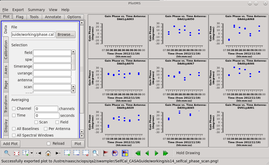
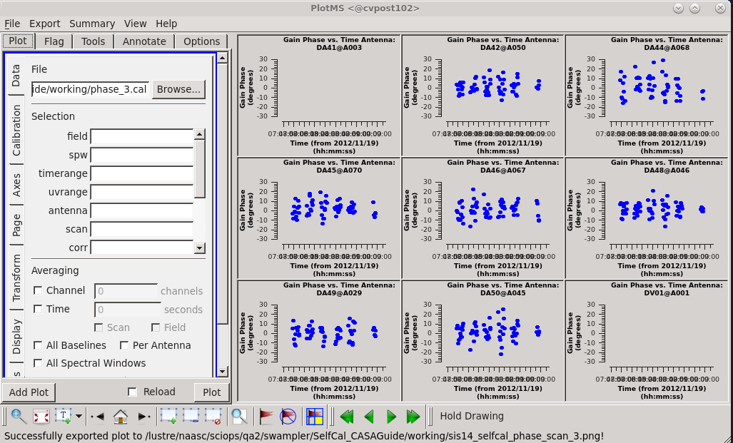
Plot the resulting solutions. We are finding nontrivial, though not enormous, solutions (a few 10s of degrees) with the two correlations tracking one another pretty well. If the data were already perfectly calibrated, these values would solve to be zero.
# In CASA
plotms(vis="phase.cal",
       xaxis="time",
       yaxis="phase",
       gridrows=3,
       gridcols=3,
       iteraxis="antenna",
       plotrange=[0,0,-30,30],
       titlefont=7,
       xaxisfont=7,
       yaxisfont=7,
       plotfile="sis14_selfcal_phase_scan.png",
       showgui = True)
We are happy with this solution. So let's apply it to the data using applycal. We only care about field 5 (the science target).
# In CASA
applycal(vis="sis14_twhya_calibrated_flagged.ms",
         field="5",
         gaintable=["phase.cal"],
         interp="linear")
At this point the self-calibrated data are stored in the MS in the "corrected data" column. Because we will want to try more rounds of self calibration, it's often useful (though not strictly necessary) at this point to split out the corrected data into a new data set. If you are restarting this tutorial, you need to first delete the output .ms and .flagversions file.
# In CASA
os.system("rm -rf sis14_twhya_selfcal.ms sis14_twhya_selfcal.ms.flagversions")
split(vis="sis14_twhya_calibrated_flagged.ms",
      outputvis="sis14_twhya_selfcal.ms",
      datacolumn="corrected")
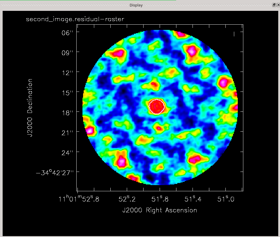
Now clean the self-calibrated data. Again, clean until the residuals on TW Hydra resemble those in the surrounding image.
# In CASA
os.system('rm -rf second_image.*')
tclean(vis='sis14_twhya_selfcal.ms',
       imagename='second_image',
       field='5',
       spw='',
       specmode='mfs',
       deconvolver='hogbom',
       nterms=1,
       gridder='standard',
       imsize=[250,250],
       cell=['0.1arcsec'],
       weighting='natural',
       threshold='0mJy',
       interactive=True,
       niter=5000,
       savemodel='modelcolumn')
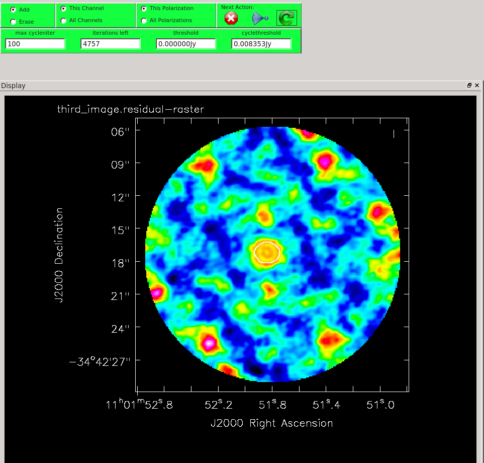
The residuals do look better this time around. Run the viewer and compare the first and second images. You should see a noticeable improvement in the noise and some improvement in the signal, so that the overall signal-to-noise (dynamic range) is much improved.
This second clean also produces a model (if the savemodel parameter is set!), hopefully a mildly better one this time.
Now we will run a second round of phase-only self calibration using the improved model.
# In CASA
os.system("rm -rf phase_2.cal")
gaincal(vis="sis14_twhya_selfcal.ms",
        caltable="phase_2.cal",
        field="5",
        solint="170s",
        calmode="p",
        refant="DV22",
        gaintype="G")
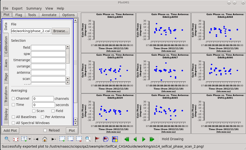
Let's plot the calibration table again. At this point, we see much smaller phase scatter relative to the model, so we don't expect more phase-only self calibration to do much.
# In CASA
plotms(vis="phase_2.cal",
       xaxis="time",
       yaxis="phase",
       gridrows=3,
       gridcols=3,
       iteraxis="antenna",
       plotrange=[0,0,-30,30],
       titlefont=7,
       xaxisfont=7,
       yaxisfont=7,
       plotfile="sis14_selfcal_phase_scan_2.png",
       showgui = True)
Apply the solutions again:
# In CASA
applycal(vis="sis14_twhya_selfcal.ms",
         field="5",
         gaintable=["phase_2.cal"],
         interp="linear")
Split the data off again. Here you can see the work flow for heavily iterative self-calibration. We progressively calibrate, split.
# In CASA
os.system("rm -rf sis14_twhya_selfcal_2.ms sis14_twhya_selfcal_2.ms.flagversions")
split(vis="sis14_twhya_selfcal.ms",
      outputvis="sis14_twhya_selfcal_2.ms",
      datacolumn="corrected")
Clean a third time.
# In CASA
os.system('rm -rf third_image.*')
tclean(vis='sis14_twhya_selfcal_2.ms',
       imagename='third_image',
       field='5',
       spw='',
       specmode='mfs',
       deconvolver='hogbom',
       nterms=1,
       gridder='standard',
       imsize=[250,250],
       cell=['0.1arcsec'],
       weighting='natural',
       threshold='0mJy',
       interactive=True,
       niter=5000,
       savemodel='modelcolumn')
# In CASA
os.system("rm -rf amp.cal")
gaincal(vis="sis14_twhya_selfcal_2.ms",
        caltable="phase_3.cal",
        field="5",
        solint="30s",
        calmode="p",
        refant="DV22",
        gaintype="T")
# Plot the amplitude solutions.
plotms(vis="phase_3.cal",
       xaxis="time",
       yaxis="phase",
       gridrows=3,
       gridcols=3,
       iteraxis="antenna",
       plotrange=[0,0,-30,30],
       titlefont=7,
       xaxisfont=7,
       yaxisfont=7,
       plotfile="sis14_selfcal_phase_scan_3.png",
       showgui = True)
# In CASA
applycal(vis="sis14_twhya_selfcal_2.ms",
         field="5",
         gaintable=["phase_3.cal"],
         interp="linear")
# In CASA
os.system("rm -rf sis14_twhya_selfcal_3.ms sis14_twhya_selfcal_3.ms.flagversions")
split(vis="sis14_twhya_selfcal_2.ms",
      outputvis="sis14_twhya_selfcal_3.ms",
      datacolumn="corrected")
Clean for a fourth time.
# In CASA
os.system('rm -rf fourth_image.*')
tclean(vis='sis14_twhya_selfcal_3.ms',
       imagename='fourth_image',
       field='5',
       spw='',
       specmode='mfs',
       deconvolver='hogbom',
       nterms=1,
       gridder='standard',
       imsize=[250,250],
       cell=['0.1arcsec'],
       weighting='natural',
       threshold='0mJy',
       interactive=True,
       niter=5000)
The improvement is really marginal at this point. Confident that we have done what we can on the phase, we can experiment with amplitude self calibration. This is potentially dangerous as it has much more potential to change the characteristics of the source than phase self-calibration. We mitigate this somewhat by setting solnorm=True, so that the solutions are normalized.
os.system("rm -rf amp.cal")
gaincal(vis='sis14_twhya_selfcal_3.ms',
        caltable="amp.cal",
        field="5",
        solint="inf",
        calmode="ap",
        refant="DV22",
        gaintype="G",
        solnorm=True)
plotms(vis="amp.cal",
       xaxis="time",
       yaxis="amp",
       gridrows=3,
       gridcols=3,
       iteraxis="antenna",
       plotrange=[0,0,0,0],
       titlefont=7,
       xaxisfont=7,
       yaxisfont=7,
       plotfile="sis14_selfcal_amp_scan.png",
       showgui = True)

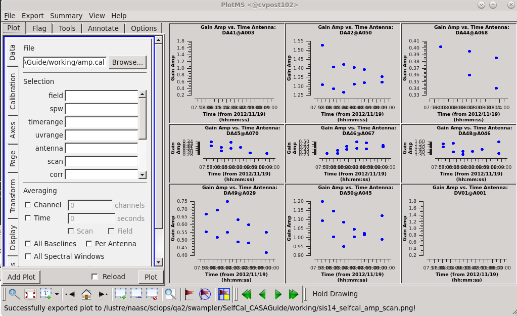
We see a good deal of scatter and some offsets between
correlations. This can be easily visualized within the plotms viewer by selecting the "Display" tab, checking the "colorize" box, and selecting "corr" to colorize the data by correlation. It is at least worth looking at what the effects of applying this will be. So let's apply these solutions on an interim basis.
applycal(vis=vis4,
         field="5",
         gaintable=["amp.cal"],
         interp="linear")
At this point the self-calibrated data live in the corrected column. Because we will want to try more rounds of self calibration, it's very useful (though not strictly necessary) at this point to split out the corrected data into a new data set.
vis5=root+'sis14_twhya_selfcal4.ms'
os.system("rm -rf "+root+"sis14_twhya_selfcal4.ms*")
split(vis=vis4,
      outputvis=vis5,
      datacolumn="corrected")
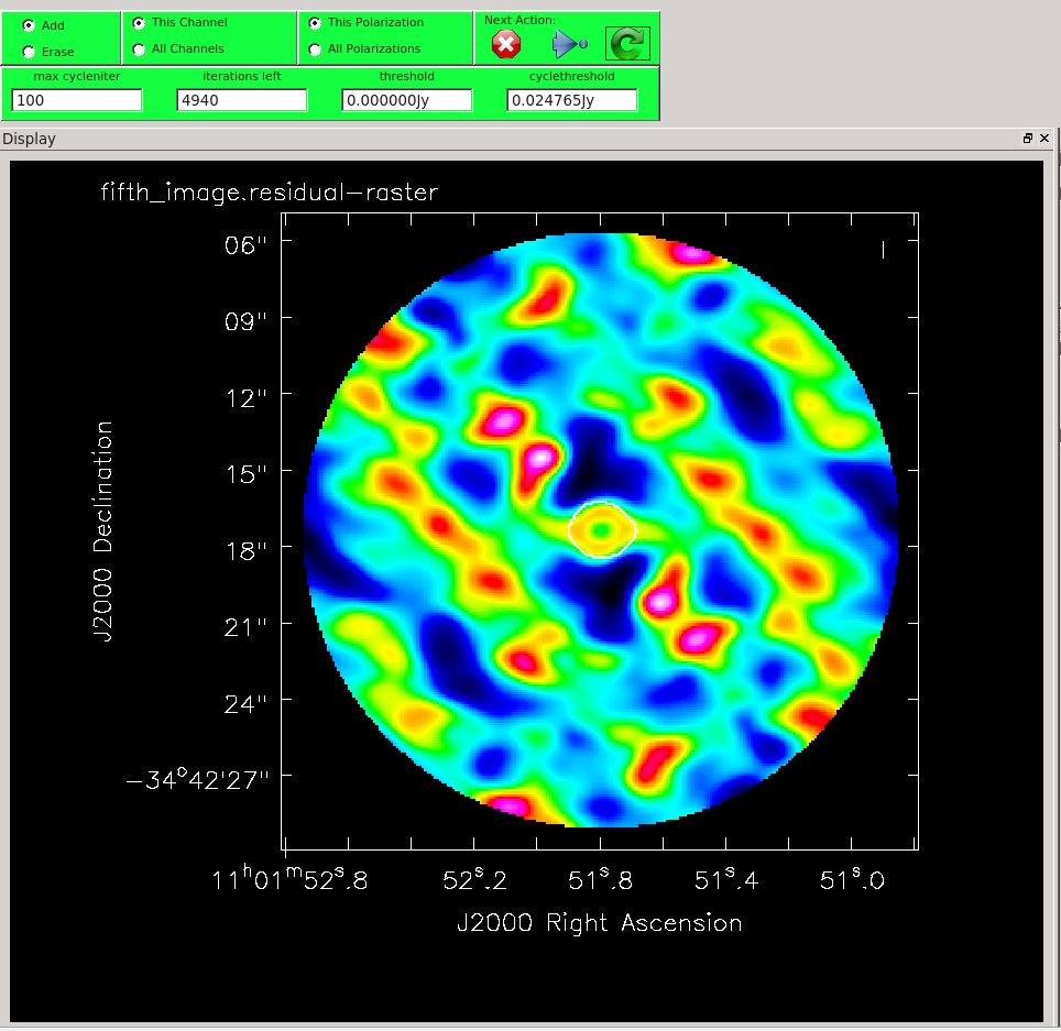
Clean a fourth time.
os.system('rm -rf fifth_image.*')
tclean(vis=vis5,
       imagename='fifth_image',
       field='5',
       spw='',
       specmode='mfs',
       deconvolver='hogbom',
       nterms=1,
       gridder='standard',
       imsize=[250,250],
       cell=['0.1arcsec'],
       weighting='natural',
       threshold='0mJy',
       interactive=True,
       niter=5000,
       savemodel='modelcolumn')
This time, notice from the residuals that you can clean more deeply. After 4 main cycles, the background residuals look very random on the scale of the beam size. This is good!
Compare the third and fourth images (you can use an imstat command or draw a box using the viewer and access the statistics panel). The noise level is dramatically better, while the flux has not changed markedly (this is very good, it's what we worry about with amplitude self calibration). By assuming that the previous cleans represent good models we have managed to improve the signal-to-noise on the data by almost an order of magnitude. Not bad!
This fourth image is our best continuum image. We can use the data set (sis14_twhya_selfcal_3.ms) to proceed with later work. In the next lesson we'll do UV continuum subtraction and line imaging.
(ASIDE: Note that you would need to do the primary beam correction on this data in the same way as you corrected the previous continuum image before making science measurements).