VLA Self-calibration Tutorial-CASA5.7.0
This page is currently under construction.
Introduction
After the initial calibration of a dataset using the observed calibrator sources, there are likely to be residual phase and/or amplitude errors in the data of the target source. Self-calibration (self-cal) is the process of using a model of the target source to reduce the phase and amplitude errors in the visibilities of the same target source. This CASA guide describes the process of self-calibration and how to choose parameters to achieve the best result.
A couple typical cases in which self-cal can help improve the image of the target source:
- Extensive artifacts from the source of interest due to calibration errors
- Extensive artifacts from a background source due to direction-independent calibration errors
Some cases in which self-cal will *not* improve the image of the target source:
- When the image artifacts are due to errors in creating the image (e.g., ignoring wide-field effects)
- When the image artifacts are due to errors in deconvolution (e.g., ignoring wide-band effects)
- When the source(s) are too weak to achieve sufficient signal-to-noise in the calibration solutions
- When there is a bright outlying source with direction-dependent calibration errors
Fundamentally, self-calibration is almost identical to standard calibration.
Both standard calibration and self-cal work by comparing the visibility data with model visibilities to solve for calibration solutions. With standard calibration, we are usually provided a model of our calibrator source by the observatory (e.g., VLA Flux-density calibrators) or we adopt a simple model (e.g., a 1 Jy point source at the phase center is a common assumption for VLA phase calibrators). With self-calibration we need to create a model of our target source, e.g., by imaging the target visibilities as we did in the above section. Then for both standard calibration and self-cal we solve for calibration solutions after making choices about the solution interval, signal-to-noise, etc. When applying the standard calibration solutions we use interpolation to correct the target, but for self-cal we apply the calibration solutions directly to the target field from which they were derived.
In this guide, we will create a model using the target data itself (using tclean), use this model to solve for and apply calibration solutions (using gaincal and applycal), then iteratively improve this model with further rounds of self-cal. This is the most common procedure, but there are other variants that are outside the scope of this guide. For example, your initial model for the target may come from fitting a model to the visibilities instead of imaging, or may be based on a priori' knowledge of the target field. Some applications of self-cal may use other calibration tasks, e.g., bandpass, instead of or in addition to gaincal.
Each "round" of self-calibration will follow the same general procedure:
- Conservatively clean the target and save the model.
- Use gaincal with a set of parameters to calculate a calibration table.
- Inspect the calibration solutions using plotms.
- Determine if the solutions should be applied, re-calculated with different parameters, or if it is time to stop.
- Use applycal to apply the table of solutions to the data.
- Use split to write out the calibrated data with the applied solutions, the starting point for the next round of self-cal.
- Start the next round of self-cal.
Note: There is an alternative and equally valid variant of the self-calibration procedure that is outlined in Appendix ... but not used in this guide.
This guide will cover:
- How to run the general self-calibration process
- How to determine optimal self-cal parameters (e.g. solution interval)
- When to stop the self-cal process
- Advanced topics related to self-cal (e.g., peeling)
Data for this Tutorial
Obtaining the Data
The dataset that will be used for this CASA tutorial is an observation of a massive galaxy cluster at z~1 which was taken with the goal of determining the morphology of the radio sources within the cluster.
The original observation has been calibrated using the VLA CASA Pipeline. It can be downloaded from the archive by searching for the following SDM name: 17B-197.sb34290063.eb34589992.58039.86119096065.
We will instruct the archive to apply the calibration solutions derived by the original pipeline execution. Therefore, the measurement set (MS) we will be downloading will contain both the raw (uncalibrated) visibilities and the calibrated visibilities, which will appear in the 'DATA' and 'CORRECTED_DATA' columns of the MS, respectively.
The raw data alone is 11.4 GB, and this will grow to 20.5 GB after applying the calibration.
As an alternative to requesting these data from the archive you may instead download the calibrated MS directly here:
-- link to data download --
A smaller data set is also available (see Section Splitting the Target Visibilities)
Observation Details
First, we will start CASA in the directory containing the data and then collect some basic information about the observation. The task listobs can be used to display the individual scans comprising the observation, the frequency setup, source list, and antenna locations.
# in CASA
listobs(vis='17B-197.sb34290063.eb34589992.58039.86119096065.ms')
A portion of the listobs output appears below:
================================================================================
           MeasurementSet Name:  17B-197.sb34290063.eb34589992.58039.86119096065.ms      MS Version 2
================================================================================
   Observer: Prof. Anthony H. Gonzalez     Project: uid://evla/pdb/34052589
Observation: EVLA
Data records: 5290272       Total elapsed time = 2853 seconds
   Observed from   13-Oct-2017/20:40:09.0   to   13-Oct-2017/21:27:42.0 (UTC)

   ObservationID = 0         ArrayID = 0
  Date        Timerange (UTC)          Scan  FldId FieldName             nRows     SpwIds   Average Interval(s)    ScanIntent
  13-Oct-2017/20:40:09.0 - 20:45:03.0     1      0 J1549+5038              550368  [0,1,2,3,4,5,6,7,8,9,10,11,12,13,14,15]  [3, 3, 3, 3, 3, 3, 3, 3, 3, 3, 3, 3, 3, 3, 3, 3] [SYSTEM_CONFIGURATION#UNSPECIFIED]
              20:45:06.0 - 20:50:03.0     2      0 J1549+5038              555984  [0,1,2,3,4,5,6,7,8,9,10,11,12,13,14,15]  [3, 3, 3, 3, 3, 3, 3, 3, 3, 3, 3, 3, 3, 3, 3, 3] [CALIBRATE_AMPLI#UNSPECIFIED,CALIBRATE_PHASE#UNSPECIFIED]
              20:50:06.0 - 20:59:27.0     3      1 MOO_1506+5136          1050192  [0,1,2,3,4,5,6,7,8,9,10,11,12,13,14,15]  [3, 3, 3, 3, 3, 3, 3, 3, 3, 3, 3, 3, 3, 3, 3, 3] [OBSERVE_TARGET#UNSPECIFIED]
              20:59:30.0 - 21:00:51.0     4      0 J1549+5038              151632  [0,1,2,3,4,5,6,7,8,9,10,11,12,13,14,15]  [3, 3, 3, 3, 3, 3, 3, 3, 3, 3, 3, 3, 3, 3, 3, 3] [CALIBRATE_AMPLI#UNSPECIFIED,CALIBRATE_PHASE#UNSPECIFIED]
              21:00:54.0 - 21:10:15.0     5      1 MOO_1506+5136          1050192  [0,1,2,3,4,5,6,7,8,9,10,11,12,13,14,15]  [3, 3, 3, 3, 3, 3, 3, 3, 3, 3, 3, 3, 3, 3, 3, 3] [OBSERVE_TARGET#UNSPECIFIED]
              21:10:18.0 - 21:11:39.0     6      0 J1549+5038              151632  [0,1,2,3,4,5,6,7,8,9,10,11,12,13,14,15]  [3, 3, 3, 3, 3, 3, 3, 3, 3, 3, 3, 3, 3, 3, 3, 3] [CALIBRATE_AMPLI#UNSPECIFIED,CALIBRATE_PHASE#UNSPECIFIED]
              21:11:42.0 - 21:21:03.0     7      1 MOO_1506+5136          1050192  [0,1,2,3,4,5,6,7,8,9,10,11,12,13,14,15]  [3, 3, 3, 3, 3, 3, 3, 3, 3, 3, 3, 3, 3, 3, 3, 3] [OBSERVE_TARGET#UNSPECIFIED]
              21:21:06.0 - 21:22:27.0     8      0 J1549+5038              151632  [0,1,2,3,4,5,6,7,8,9,10,11,12,13,14,15]  [3, 3, 3, 3, 3, 3, 3, 3, 3, 3, 3, 3, 3, 3, 3, 3] [CALIBRATE_AMPLI#UNSPECIFIED,CALIBRATE_PHASE#UNSPECIFIED]
              21:22:30.0 - 21:27:03.0     9      2 3C286                   511056  [0,1,2,3,4,5,6,7,8,9,10,11,12,13,14,15]  [3, 3, 3, 3, 3, 3, 3, 3, 3, 3, 3, 3, 3, 3, 3, 3] [CALIBRATE_BANDPASS#UNSPECIFIED,CALIBRATE_FLUX#UNSPECIFIED]
              21:27:06.0 - 21:27:42.0    10      2 3C286                    67392  [0,1,2,3,4,5,6,7,8,9,10,11,12,13,14,15]  [3, 3, 3, 3, 3, 3, 3, 3, 3, 3, 3, 3, 3, 3, 3, 3] [CALIBRATE_BANDPASS#UNSPECIFIED,CALIBRATE_FLUX#UNSPECIFIED]
           (nRows = Total number of rows per scan)
Fields: 3
  ID   Code Name                RA               Decl           Epoch   SrcId      nRows
  0    NONE J1549+5038          15:49:17.468534 +50.38.05.78820 J2000   0        1561248
  1    NONE MOO_1506+5136       15:06:20.353700 +51.36.53.63460 J2000   1        3150576
  2    NONE 3C286               13:31:08.287984 +30.30.32.95886 J2000   2         578448
Spectral Windows:  (16 unique spectral windows and 1 unique polarization setups)
  SpwID  Name           #Chans   Frame   Ch0(MHz)  ChanWid(kHz)  TotBW(kHz) CtrFreq(MHz) BBC Num  Corrs
  0      EVLA_C#A0C0#0      64   TOPO    4488.000      2000.000    128000.0   4551.0000       12  RR  RL  LR  LL
  1      EVLA_C#A0C0#1      64   TOPO    4616.000      2000.000    128000.0   4679.0000       12  RR  RL  LR  LL
  2      EVLA_C#A0C0#2      64   TOPO    4744.000      2000.000    128000.0   4807.0000       12  RR  RL  LR  LL
  3      EVLA_C#A0C0#3      64   TOPO    4872.000      2000.000    128000.0   4935.0000       12  RR  RL  LR  LL
  4      EVLA_C#A0C0#4      64   TOPO    5000.000      2000.000    128000.0   5063.0000       12  RR  RL  LR  LL
  5      EVLA_C#A0C0#5      64   TOPO    5128.000      2000.000    128000.0   5191.0000       12  RR  RL  LR  LL
  6      EVLA_C#A0C0#6      64   TOPO    5256.000      2000.000    128000.0   5319.0000       12  RR  RL  LR  LL
  7      EVLA_C#A0C0#7      64   TOPO    5384.000      2000.000    128000.0   5447.0000       12  RR  RL  LR  LL
  8      EVLA_C#B0D0#8      64   TOPO    5488.000      2000.000    128000.0   5551.0000       15  RR  RL  LR  LL
  9      EVLA_C#B0D0#9      64   TOPO    5616.000      2000.000    128000.0   5679.0000       15  RR  RL  LR  LL
  10     EVLA_C#B0D0#10     64   TOPO    5744.000      2000.000    128000.0   5807.0000       15  RR  RL  LR  LL
  11     EVLA_C#B0D0#11     64   TOPO    5872.000      2000.000    128000.0   5935.0000       15  RR  RL  LR  LL
  12     EVLA_C#B0D0#12     64   TOPO    6000.000      2000.000    128000.0   6063.0000       15  RR  RL  LR  LL
  13     EVLA_C#B0D0#13     64   TOPO    6128.000      2000.000    128000.0   6191.0000       15  RR  RL  LR  LL
  14     EVLA_C#B0D0#14     64   TOPO    6256.000      2000.000    128000.0   6319.0000       15  RR  RL  LR  LL
  15     EVLA_C#B0D0#15     64   TOPO    6384.000      2000.000    128000.0   6447.0000       15  RR  RL  LR  LL
Initial Data Inspection
Since we have obtained the calibrated visibilites for the calibrator fields, we can now take this opportunity to investigate at high signal-to-noise the magnitude and timescale of the phase fluctuations we will be trying to correct for with selfcal.
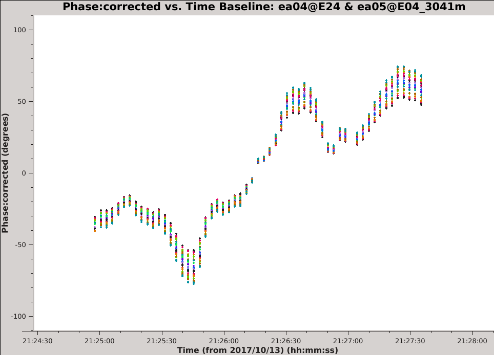
Looking at the output of listobs we see that there is a long scan on the amplitude calibrator, 3C 286 (field ID 2). We will plot the calibrated phase vs. time on a single baseline:
# in CASA
plotms(vis='17B-197.sb34290063.eb34589992.58039.86119096065.ms', xaxis='time', yaxis='phase', ydatacolumn='corrected', field='2', antenna='ea05', correlation='RR,LL', avgchannel='64', iteraxis='baseline', coloraxis='spw')
- vis='17B-197.sb34290063.eb34589992.58039.86119096065.ms' : To plot visibilities from the pipeline calibrated MS.
- xaxis='time', yaxis='phase' : To set time as the x-axis and phase as the y-axis of the plot.
- ydatacolumn='corrected' : To plot the calibrated data (from the CORRECTED_DATA column).
- field='2' : To select visibilities from field ID 2, i.e., the amplitude calibrator 3C 286.
- antenna='ea05', iteraxis='baseline' : To view a single baseline at a time.
- correlation='RR,LL' : To plot both parallel-hand correlation products.
- avgchannel='64' : To average all channels in each SPW to increase signal-to-noise. Since the bandpass solutions have been applied to these data the channels will average coherently.
- coloraxis='spw' : To plot each SPW as a different color, which will make it easier to distinguish them.
Use the 'Next Iteration' button of the plotms GUI to cycle through additional baselines. You should see plots that look similar to the example image of the ea04-ea05 baseline. The plotted data have a mean of zero phase because the pipeline calibration solutions have already been applied. The phase is seen to vary with time over a large range (in some cases more than +/- 100 degrees) and the variations appear to be smooth over time scales of a few integrations. All of the spectral windows and both correlations follow the same trend with time. Additionally, the magnitude of the phase variations is larger for the higher frequency spectral windows, a pattern that is consistent with a change in atmospheric density.
Optional extra steps: Create and inspect similar plots using scan 2 of the phase calibrator field (J1549+5038). Repeat for baselines to other antennas.
Splitting the Target Visibilities
It is essential that we split the calibrated visibilities for the target we want to self-calibrate, meaning that the visibilities of the target source get copied from the CORRECTED_DATA column of the pipeline calibrated MS to the DATA column of a new measurement set. CASA calibration tasks always operate by comparing the visibilities in the DATA column to the source model, where the source model is given by either the MODEL_DATA column, a model image or component list, or the default model of a 1 Jy point source at the phase center. In the same way that the calibration pipeline used the raw visibilities in the DATA column to solve for calibration tables and then created the CORRECTED_DATA column by dividing the DATA column by these tables, self-calibration will work by comparing the pipeline calibrated visibilities (in the DATA column of the split MS) to a model, solving for self-calibration tables, and then creating a new CORRECTED_DATA column by applying the self-calibration tables.
# in CASA
split(vis='17B-197.sb34290063.eb34589992.58039.86119096065.ms',datacolumn='corrected',field='1', correlation='RR,LL', outputvis='obj.ms')
- vis='17B-197.sb34290063.eb34589992.58039.86119096065.ms' : The input visibilities for split. Here, these are the visibilities produced by the pipeline.
- datacolumn='corrected' : To copy the calibrated visibilities from the input MS.
- field='1' : The field ID of the target we want to self-calibrate.
- correlation='RR,LL' : To select only the parallel hand correlations. This will make the output data set smaller by about a factor of two.
- outputvis='obj.ms' : The name of the new measurement set that split will create.
-- The output MS can be can be directly downloaded here: obj.ms (3.4 GB) --
Initial Imaging
Prior to solving for self-calibration solutions we need to make an initial model of the target field. We will generate this model by deconvolving the target field using the task tclean. But before doing so, there are several imaging considerations that we should address prior to making this model (discussed below):
Image field-of-view: Ideally, we want our self-calibration model to include all of the sources present in the data (e.g., sources near the edge of the primary beam or in the first sidelobe). This is typically achieved by making an image large enough to encompass all of the apparent sources, or by making a smaller image of the target plus one or more outlier fields. We will start with a large dirty image of the entire primary beam (PB) in order to better understand the sources in the galaxy cluster plus any background sources that will need to be cleaned. A rule of thumb for the VLA is that the FWHM of the PB in arcminutes is approximately 45 * (1 GHz / nu). For our C-band observations, the VLA primary beam is ~8' FWHM. In order to image the entire PB and the first sidelobe we need an image field of view that is about four times larger, so we will choose a 32' field-of-view for our initial image. (see ... for a more complete discussion of the calculation of primary beam sizes)
Image cell size: There are a few different ways to estimate the synthesized beam size for these observations taken with the C-band in the B-configuration. For one, we can use this table in the VLA Observational Status Summary, which gives a resolution of 1.0" (see ... for a more complete discussion of the calculation of synthesized beam sizes). It is recommended to choose a cell size that will result in at least 5 image pixels across the FWHM of the synthesized beam, therefore we require a cell size of 0.20"/pixel or smaller.
Image size in pixels: We can convert our desired field-of-view to pixels using the cell size: 32' * (60" / 1') * (1 pixel / 0.20") = 9600 pixels. However, when making large images, CASA will run faster if we choose an image size that is optimized for the FFT algorithm. The recommendation is to choose an image size that can be expressed as 5*2^n*3^m. This is so that after CASA applies an internal padding factor of 1.2, the images being used in the FFTs can be broken down into small 2x2 and 3x3 matrices. So we will choose an optimized image size of 9720 (n=3,m=5) for this image.
Wide-field effects: Large images may require additional consideration due to non-coplanar baselines (the W-term). In CASA, this is usually addressed by turning on the W-project algorithm. See this link to CASAdocs for a more detailed discussion.
We can estimate whether our image requires W-projection by calculating the recommended number of w-planes using this formula taken from page 392 of the NRAO 'white book',
[math]\displaystyle{ N_{wprojplanes} = \left ( \frac{I_{FOV}}{\theta_{syn}} \right ) \times \left ( \frac{I_{FOV}}{1\, \mathrm{radian}} \right ) }[/math]
where I_FOV is the image field-of-view and theta_syn is the synthesized beam size. This evaluates to wprojplanes ~ 18 so we will choose to turn on the w-project algorithm with gridder='widefield' and set wprojplanes=18.
We will now create the initial dirty image using these parameters.
# in CASA
tclean(vis='obj.ms',imagename='obj.dirty.9720pix',imsize=9720, cell='0.2arcsec', pblimit=-0.1, gridder='widefield', wprojplanes=18 )
- cell='0.2arcsec': The size of an image pixel (see above).
- imsize=9720: The number of pixels across one side of the (square) image.
- pblimit=-0.1: We set this to a small negative number to turn off the PB mask.
- gridder='widefield': To turn on the w-project algorithm.
- wprojplanes=18: The number of w-planes to use for w-projection.
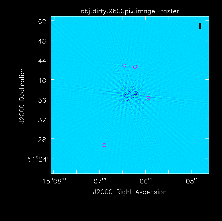
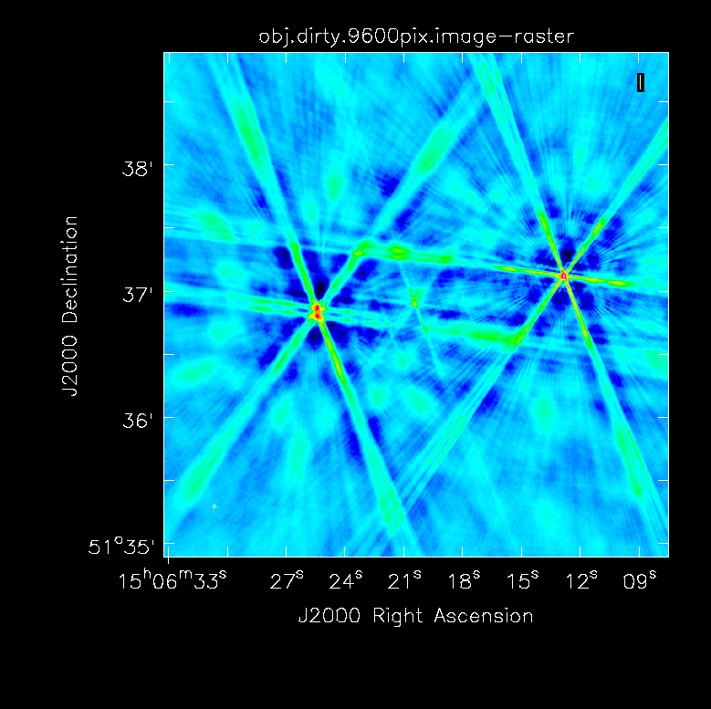
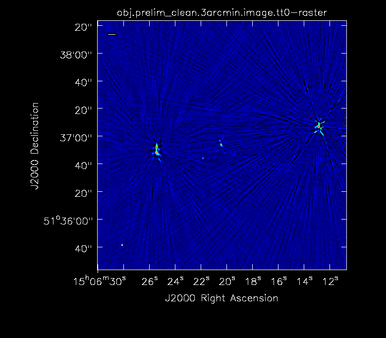
Figure 2A below shows the resulting dirty image, and Figure 2B shows a zoom-in of the central region of the image. Several outlying sources are detectable; the four brightest are marked with magenta circles.
We have a few options about how to deal with these outlying sources:
- Proceed with the self-calibration procedure using a large field-of-view that includes all the outlying sources.
- Proceed with the self-calibration procedure using a small field-of-view that includes only the central sources, and add an outlier field on each of the outlying sources.
- Model and UV-subtract the outlying sources.
- Peel the outlying sources.
- Proceed with the self-calibration procedure using a small field-of-view that includes only the central sources, ignoring the outlying sources.
In this guide, we will first choose to ignore the outlying sources in order to present a simplified self-calibration procedure. At the end of this guide, we will re-visit this choice and show examples of more advanced procedures.
Initial Model
After deciding how to deal with the outlying sources, our next step is to make the initial model that we will use for self-calibration. There are a few additional parameters that apply to this step, discussed below.
Image field-of-view: For this science case we are only interested in sources within ~1.5' of the cluster center. Since we have chosen to ignore the outlying sources at this stage, we will proceed with an image field-of-view of 3'.
Wide-field effects: We repeat the calculation of wprojplanes from the Initial Imaging section, which results in wprojplanes ~ 1. Therefore, we turn off the correction for non-coplanar baselines by setting gridder='standard' .
Wide-band imaging: Our images will combine data from all spectral windows, spanning a frequency range of about 4.5-6.5 GHz (a fractional bandwidth of about 36%). Each source's amplitude may vary substantially over this frequency range, due to either the source's intrinsic spectral variation and/or the frequency dependence of the VLA's primary beam. To mitigate these errors during deconvolution we will use deconvolver='mtmfs' and nterms=2. For further discussion of wide-band imaging, see the CASA documentation for wide-band imaging and the VLA Imaging CASAguide.
Imaging weights: When constructing the initial model, especially when there are large image artifacts, it is recommended to use "robust" imaging weights. In CASA, this is enabled with weighting='briggs' , and then choosing a value for the robust parameter. Large positive values of robust often result in large positive PSF sidelobes while large and negative values of robust often produce large negative PSF sidelobes. Since many types of image artifacts scale with PSF sidelobe levels, a reasonable compromise is often around robust=0.
Image deconvolution: We will need to deconvolve (clean) this image in order to produce a model of the field. We will want to control the cleaning depth and masking interactively, so we set interactive=True. We also must choose the number of clean iterations with the niter parameter-- 1000 iterations is a suggested starting value, and this can be changed interactively after we start cleaning.
Saving the model: After deconvolution, there are a couple options for how to save the model, controlled by the savemodel parameter. The default is none which will not save the model. It is essential that this default is changed or else the selfcal procedure will fail. The option savemodel='virtual' will save a copy of the image to the SOURCE subtable of the measurement set to be used later for on-the-fly model visibility prediction. This option is sometimes recommended for very large data sets. The other option, savemodel='modelcolumn' is the recommended setting and the one that we will use in this guide. This option will do the model visibility prediction after cleaning and save the result to the MODEL_DATA column.
Now we are ready to create our first clean image. This image will provide the starting model that is required by the calibration routines, and it will showcase why we need self-calibration for these data.
# in CASA
tclean(vis='obj.ms',imagename='obj.prelim_clean.3am', gridder='standard', cell='0.2arcsec', imsize=900, pblimit=-0.1, deconvolver='mtmfs', nterms=2, niter=1000, interactive=True, weighting='briggs', robust=0, savemodel='modelcolumn')
- gridder='standard': We select the default gridder (assumes coplanar baselines).
- cell='0.2arcsec': The size of an image pixel.
- imsize=900: To create an image with a 3' field-of-view.
- pblimit=-0.1: To remove the PB mask; see previous sections.
- deconvolver='mtmfs': We will turn on the wide-band deconvolution algorithm as discussed above.
- nterms=2: The number of Taylor terms for wide-band deconvolution.
- niter=1000: Set a relatively large number of iterations as a starting point.
- interactive=True: So we can interactively place the mask.
- weighting='briggs': Turn on 'robust' image weighting
- robust=0: Set the value of the robust weighting.
- savemodel='modelcolumn': To enable writing the MODEL_DATA column after imaging. **important**
During the interactive cleaning, we place circular masks around each of the strong sources in turn:
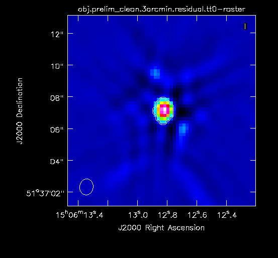
- The rightmost source (Figure 2A) -- let it run the first set of clean iterations by pressing the green circle arrow in the CASA viewer.
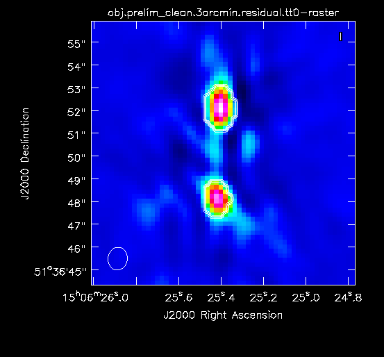
- The leftmost double-lobed source (Figure 2B) -- let it run an additional set of clean iterations by pressing the green circle arrow in the CASA viewer.
- The middle source (Figure 2C) -- continue cleaning inside the masks by pressing the green circle arrow in the CASA viewer.
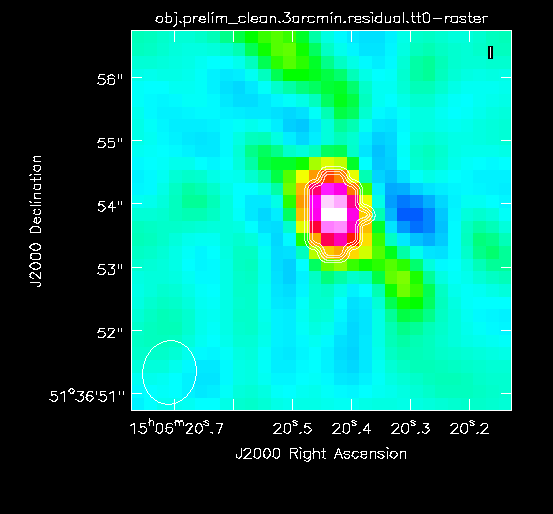
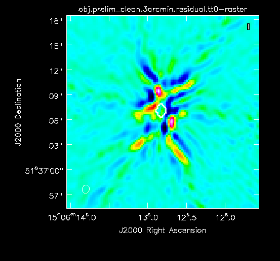
At this point, the residual emission is at about the same level as the artifacts so we stop cleaning (a total of about 225 iterations; see Figure 2D for an example of the artifacts). It is strongly recommended to only mask and clean emission that is believed to be real so as not to include artifacts in the model. Figure 2E shows the resulting clean image that we will try to improve through the use of self-calibration.
Verifying the Initial Model
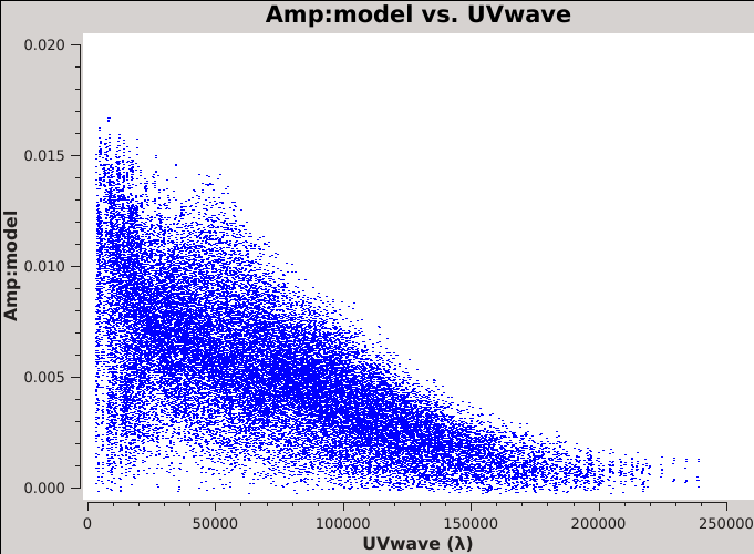
There have been reported instances where CASA fails to save the model visibilities when using interactive clean. It is crucial that the model is saved correctly, otherwise self-calibration will use the 'default' model of a 1 Jy point source at the phase center. The default model may be very different from your target field and we do not want to carry out the self-cal procedure with this incorrect model. Therefore, it is recommended to verify that the model has been saved correctly by inspecting the model visibilities.
# in CASA
plotms(vis='obj.ms', xaxis='UVwave', yaxis='amp', ydatacolumn='model', correlation='RR,LL', avgchannel='64', avgtime='300s')
- vis='obj.ms' : To plot visibilities from the split MS.
- xaxis='UVwave', yaxis='amp' : To set UV-distance in wavelengths as the x-axis and amplitude as the y-axis of the plot.
- ydatacolumn='model' : To plot the model visibilities (from the MODEL_DATA column).
- correlation='RR,LL' : To only plot the parallel-hand visibilities. The model RL=LR=0 since we only made a Stokes I model image.
- avgchannel='64' : To average all channels per SPW.
- avgtime='300s' : To average in time in chunks of 300 seconds.
The resulting plot should resemble Figure 3 on the right. This plot shows that some baselines see up to 15 mJy of flux, but that the source becomes resolved on the longer baselines.
This model that has been plotted is clearly not the default model of a 1 Jy point source and so we have verified that tclean has correctly written the MODEL_DATA column.
First Round of Self-Calibration
For this first round of self-cal we will use the model that we just created above, so we are now ready to solve for the first self-cal solutions. We will first explore various parameters of the task gaincal in order to learn more about the data and settle on the optimal parameters. The most relavant parameters are discussed below:
Solution interval: This is controlled with the solint parameter and is one of the most fundamental parameters for self-calibration. The value of this parameter can vary between 'int' for a single integration (corresponding to 3 seconds for this data set) up to 'inf' for infinite (meaning an entire scan or the entire observation, depending on the value of the combine parameter) . We typically want to choose the shortest solution interval for which we can achieve adequate signal-to-noise in the calibration solutions.
Data combination: The data can be combined in multiple ways to improve signal-to-noise, but if the target source is bright enough to obtain good calibration solutions in a short timescale without data combination then these options need not be used. One can try to combine multiple SPWs with combine='spw' if the SPWs are at similar frequencies, and can generally expect to increase the solution's signal-to-noise by the square root of the number of SPWs that are combined. Both parallel-hand corrleations, if present, can be combined by setting gaintype='T' instead of gaintype='G' and this will generally increase the signal-to-noise by a factor of root 2. Combining scans is not usually recommended.
Amplitude and phase calibration: Because large phase errors will result in incoherent averaging and lead to lower amplitudes, we always want to start with phase-only self-calibration. We achieve this by setting calmode='p' . In later rounds of self-cal, after the phases have been well corrected, we can try calmode='ap' to include an amplitude component to the solutions. We may also want to consider normalizing the amplitudes using the solnorm parameter.
Reference antenna: As with standard calibration, we want to choose a reference antenna for the calibration solutions. One that is near the center of the array, but not flagged due to shaddowing, is generally recommended.
Next, we investigate which solution interval (solint) is optimal for this particular dataset. We will do this by generating and viewing the corrections calculated over several solution intervals (namely on the order of the integration time, 15 seconds, and 45 seconds) using gaincal.
# in CASA
gaincal(vis='obj.ms',caltable='sc1_tb_int',solint='int',refant='ea24',calmode='p',gaintype='T')
- caltable='sc1_tb_int':'Name the calibration tables something intuitive to distinguish each one. In this case, sc1 for self-calibration round 1, tb for table, and int for a solution interval of the integration time.
- solint='int': For this first calibration table, we choose the solutions to be calculated on the level of the integration time (3 seconds in this case) in order to get a sense of the structure and durations of the variations.
- refant='ea24': Choose a reference antenna that is near the center of the array but not the exact center (Josh: I think that is why we chose this one?). In order to view what antennas are near the center use plotants.
- calmode='p': Start with phase only calibration as that is where the most gain is to be had (there is a way more technical way to say that).
- gaintype='T': It is often a good idea to combine the polarizations to understand the overall data.
To view these solutions, we use plotcal.
# in CASA
plotcal(caltable='sc1_tb_int.gain',xaxis='time',yaxis='phase',iteration='antenna',subplot=321)
- xaxis='time' & yaxis='phase': View the phase variations over time with respect to antenna 24.
- iteration='antenna': View the corrections for each antenna.
- subplot=321: It can be helpful to view multiple plots at once, as we will be scrolling through the solutions for each antenna. In this case, 3 rows and two columns.
Show examples of a few of these. gaincal calculates the gains for each antenna/spwid are determined from the ratio of the data column (raw data), divided by the model column, for the specified data selection.(Josh: a bit more about technically what we are looking at and how they affect the data? -- these are the variations in phase between pairs of antennas which can cause the artifacts?) Each color represents a different spectral window. There is definitely structure we want to correct for. We use this solint = int to get a sense of on what time scale the variations occur and the amplitude of the variations. Use the zoom in feature to zoom in on these variations and estimate what the time interval of these variations are. The solint of int shows the variations, but we postulate that a 15 second or 45 second interval would catch these overall variations better.
# in CASA
gaincal(vis='obj.ms',caltable='sc1_tb_15s',solint='15s',refant='ea24',calmode='p',gaintype='T')
gaincal(vis='obj.ms',caltable='sc1_tb_45s',solint='45s',refant='ea24',calmode='p',gaintype='T')
Images of both of these. Comparing the two, we see that they both encapsulate the structure of the variations, however solint=15s encapsulates the variations the best. Thus we choose to apply sc1_tb_15s.gain. Note the amplitude of these variations in sc1_tb_15s.gain; they are typically up to 40 degrees and -60 yo -80 degrees.
Apply Calibration
# in CASA
applycal(vis='obj.ms',gaintable='sc1_tb_15s.gain')
Other potential intervals that could be useful to use are 5 seconds and 60 seconds. Additionally, if the plotcal reveals no structure in these intervals, you can combine the spws together and apply a combined solution by setting combine='spw' (you will have to set spwmap=[0 x number of spectral windows] in apply cal in order to tell CASA to apply the combined solution to all of the spectral windows -- in this case spwmap = [0,0,0,0,0,0,0,0,0,0,0,0,0,0,0,0])
Our goal is to create a better model of the source using the data itself to create a better image. The process with calculating corrections and applying them has (if done correctly) reduced the errors allowing us to make a better image and create a better model. applycal applies the solutions to the (raw) MS DATA column and writes the calibrated data into the CORRECTED_DATA column, thus for determining the next order/level of corrections during the next round of calibration we need to make the corrected data column the data column.
# in CASA
split(vis='obj.ms',outputvis='sc1_obj.ms')
Second Round of Self-Calibration
We will go through the same process again: image, gaincal, applycal, and image. This time the image we create at first will be an indication if the solutions we applied made a difference.
# in CASA
tclean(vis='obj.ms',imagename='obj.sc1',imsize=750,cell='0.24arcsec',weighting='briggs',deconvolver='mtmfs',niter=500,savemodel='modelcolumn',interactive=True)
Larger mask.
# in CASA
gaincal(vis='obj.ms',caltable='sc2_tb_15s',solint='15s',refant='ea24',calmode='p',gaintype='T')
- solint='15s': Since we found a good interval of 15 seconds previously, we move forward with 15s.
Josh: do we want to suggest/show other solution intervals? Do we want to comment on using various intervals -- when is it useful to do several rounds with one interval versus several rounds with each a different solint?
View the solutions.
# in CASA
plotcal(caltable='sc1_tb_int.gain',xaxis='time',yaxis='phase',iteration='antenna',subplot=321)
We can see our corrections made a difference. In particular notice the amplitude of the phase variations, instead of +_60-80 degress they are fractions of a degree. This indicates that we have corrected for a majority of the variations.
When to stop: (looking at amplitude of corrections, image has improved/dynamical range)
Notes about amplitude corrections (?) (mode='ap' or 'a').
When self-cal helped, but didn't improve the image enough: (suggestions for other things to do)
Appendix
PB calculations
PSF calculations
Note: There is an alternative and equally valid variant of the self-calibration procedure that is outlined below but not used in this guide. This variant avoids the use of split to freeze-in the self-cal solutions and instead builds up a list containing the calibration table(s) from each round of self-cal.
- Conservatively clean the target and save the model.
- Use gaincal with a set of parameters to calculate a calibration table, pre-applying all previous self-cal tables 'on-the-fly' with the gaintable parameter.
- Inspect the new calibration solutions using plotms.
- Determine if the solutions should be applied, re-calculated with different parameters, or if it is time to stop.
- Append the new solutions to the list of calibration tables.
- Use applycal to apply the list of tables to the data.
- Start the next round of self-cal.
