Simulating ngVLA Data-CASA5.4.1
Introduction
The following tutorial shows how to create simulated data for the next generation Very Large Array (ngVLA). The ngVLA is composed of different subarrays that make up the current reference design. The configuration files for the different subarrays are found in the "ngVLA Configuration Tools" and it be included in CASA distributions 5.5 and greater. They can be used for simulations and calculations that investigate the scientific capabilities of the ngVLA. Each configuration (.cfg) file contains the name of the observatory, the antenna positions, the coordinate system of the antenna positions and the diameter and pad name of each antenna. For these configuration files, the coordinate system is 'global', which signifies that the positions x, y, z are in meters relative to the Earth center following the FITS WCS convention.
CASA provides two ways to create a simulation: the simobserve task and the sm toolkit. With these methods we can generate measurement sets, add thermal noise and predict model visibilities, from which we can explore the ngVLA’s imaging capabilities. The simobserve task is very user friendly but it is important to be aware that it has several limitations and it has been designed primarily for ALMA and EVLA. For this reason we also demonstrate the use of the sm toolkit, which provides much more flexibility in setting the observational parameters and is more compatible with observatories that are not recognized by CASA.
In this tutorial we present three example simulations: (i) simobserve using a model image, (ii) simobserve using a component list, and (iii) a sm toolkit simulation. For more information about component lists, see the CASA guides "here" and "here". The model image used in portions of this guide, "a 93 GHz model of a protoplanetary disk, can be downloaded here". We will also show how to create and use a component list instead of a model image for the simulations. We will create example continuum simulations at 93 GHz, consisting of a single channel observed for a total of 4 hours with a 60 second integration time† . We will then add to these simulations an amount of thermal noise that is representative of the ngVLA's continuum sensitivity. The array configuration used in this guide is the Main ngVLA subarray, which is composed of 214 18 m antennas and extends over a maximum baseline of 1005.4 km. The configuration file that we will use throughout this tutorial is called ngvla-main-revC.cfg and it can be found "here".
† We choose this integration time in order to keep the measurement set files small. Time smearing is not an issue for simulated observations, but this value would need to be reconsidered before scheduling actual observations.
Estimating the scaling parameter for adding thermal noise
Simobserve's parameter to corrupt the simulated data is called thermalnoise and for interferometric data the allowed values are "tsys-atm", "tsys-manual" or " " (see this "CASA guide" for more details). The option " " will not add any noise to the data, and the option "tsys-atm" is only applicable to ALMA since it uses site parameters which are specific to that observatory. For the option "tsys-manual", it is necessary to supply several additional parameters which are required to construct an atmospheric model. In order to achieve the desired sensitivity without atmospheric modeling, we have chosen to corrupt the simulated data using the "sm.setnoise" function of the sm toolkit. In addition to the modes "tsys-atm" and "tsys-manual", this function also allows the option of "simplenoise". As the name indicates, "simplenoise" adds random Gaussian noise to the visibilities based on a simple scaling factor. We will use this same technique for all three example simulations, i.e., those made with the simobserve task and those made with the sm toolkit.
In order to estimate the scaling factor for the "simplenoise" parameter in sm.setnoise we use the following procedure:
The RMS noise ([math]\displaystyle{ \sigma_{NA} }[/math]) in an untapered, naturally-weighted Stokes I image will be approximately (see "setnoise function")
[math]\displaystyle{ \sigma_{NA} \sim \frac{\sigma_{simple}}{ \sqrt{n_{ch}\,n_{pol}\,n_{baselines}\,n_{integrations} }} }[/math] (1)
where [math]\displaystyle{ \sigma_{simple} }[/math] is the simplenoise parameter in sm.setnoise and corresponds to the noise per visibility, [math]\displaystyle{ n_{ch} }[/math] is the total number of channels across all spectral windows, [math]\displaystyle{ n_{pol} }[/math] is the number of polarizations used for Stokes I (typically 2) and [math]\displaystyle{ n_{integrations} }[/math] is the number of correlator integration times in the measurement set (i.e., total on-source time / integration time). For the example simulations in this gude, the track time is 4 h and the integration time is 60 s, thus [math]\displaystyle{ n_{integrations}=240 }[/math]. Additionally, for these examples the total number of channels is 1 and the number of polarizations is 2. The number of baselines [math]\displaystyle{ n_{baselines} }[/math] is [math]\displaystyle{ N(N-1)/2 }[/math] where N is the number of antennas in the array. For the array configuration used in this guide (ngvla-main-revC.cfg), N=214 and therefore [math]\displaystyle{ n_{baselines}= 22791 }[/math].
If you already know the expected image noise ([math]\displaystyle{ \sigma_{NA} }[/math]) for your untapered, naturally-weighted image, you can solve for the scaling parameter [math]\displaystyle{ \sigma_{simple} }[/math] in the above equation (1) and pass [math]\displaystyle{ \sigma_{simple} }[/math] to the simplenoise parameter in sm.setnoise.
If instead you want to calculate the expected sensitivity for an ngVLA image we suggest the below procedure:.
(i) Calculate the expected untapered, naturally weighted point source sensitivity ([math]\displaystyle{ \sigma_{NA} }[/math]) using one of the ngVLA performance tables. In Appendix D of "ngVLA memo #55 " there are key performance metrics for 6 subarrays which are tabulated as a function of frequency and resolution. For our example, we find in Table 10 of ngVLA memo #55 that the untapered, naturally weighted point source sensitivity of the Main interferometric array at 93 GHz is 0.83 uJy/beam for a 1 hour observation.
(ii) Scale that number to the desired observation length, in this case [math]\displaystyle{ t_{track}=4\,h }[/math]. Therefore, [math]\displaystyle{ \sigma_{NA} = 0.83/\sqrt{(t_{track}/1\,hour)} = 0.415\,\text{uJy/beam} }[/math].
(iii) Use the expected image noise ([math]\displaystyle{ \sigma_{NA} }[/math]) in the above equation (1) to solve for the scaling factor [math]\displaystyle{ \sigma_{simple} }[/math]. In this case, [math]\displaystyle{ \sigma_{simple}=0.415*\sqrt{1*2*22791*240} = 1.4\,\text{mJy} }[/math].
Once you have derived the scaling factor [math]\displaystyle{ \sigma_{simple} }[/math], run sm.setnoise and corrupt the visibilities of the noise-free measurement set. Your resulting untapered, naturally-weighted image will then have an RMS approximately equal to your desired image noise. Since it is not easy to undo this step, it is a good idea to make a copy of the noise-free measurement set before adding noise. The following mock example outlines this procedure:
# In CASA
## create a copy of the noise-free MS
os.system('cp -r noise_free.ms noisy.ms')

## open the MS we want to add noise to with the sm tool
sm.openfromms('noisy.ms')

## set the noise level using the simplenoise parameter estimated in Section: "Estimating the scaling parameter for adding thermal noise"
sm.setnoise(mode = 'simplenoise', simplenoise = sigma_simple)

## add noise to the 'DATA' column (and the 'CORRECTED_DATA' column if present)
sm.corrupt()

## close the sm tool
sm.done()
Note that this example will not execute without a measurement set named "noise_free.ms" and a defined variable sigma_simple. See below for working examples of this procedure used in conjunction with the creation of simulated measurement sets and the prediction of model visibilities.
Example simulation using Simobserve with a model image
We will use the simobserve task to create our first noise-free measurement set (MS), using the configuration file and model image described in the Introduction.
# In CASA

simobserve(project = 'ngVLA_214_ant_60s_noise_free',
                    skymodel = 'ppmodel_image_93GHz.fits',
                    setpointings = True,
                    integration = '60s',
                    obsmode = 'int',
                    antennalist = 'ngvla-main-revC.cfg',
                    hourangle = 'transit',
                    totaltime = '14400s',
                    thermalnoise = '',
                    graphics = 'none')
project: Simobserve will create a folder with the project name in your current working directory, and this folder will contain all the resulting files including the noise-free MS.
skymodel: The input model image in Jy/pixel units, which can be a single image or a spectral cube. The simulated MS will inherit the number of channels, central frequency, source direction and peak flux of this input model. These can be adjusted using the optional parameters inbright, indirection, incell, incenter and inwidth. In this example we do not modify these optional parameters.
setpointings: We choose the value of True, which allows simobserve to derive the pointing positions using its own algorithm and properties of the input model image. Since the size of the model is much smaller than the primary beam, a single pointing will be generated (instead of a mosaic). We also set the expanded parameter integration to '60s' (our chosen correlator integration time) and leave other expanded parameters set to their default values.
obsmode: We set this parameter to 'int' to simulate interferometric data. We also set values for several expandable parameters. For antennalist we give the name of the configuration file for the ngVLA Main interferometric array. simobserve will read this file from a directory inside the CASA distribution (casa.values()[0]['data']+'/alma/simmos/') if you are using CASA version 5.5 or greater. We set totaltime to the total on-source observation time, use the hourangle parameter to center our observation time on transit, and leave other expanded parameters as default.
thermalnoise: We leave this parameter empty to create a noise-free simulation. We will add the noise later in a separate step (see below).
graphics: This will show graphics on the screen and/or save them as png files in the project directory. However, at the moment this is not working properly for baselines larger than a few hundred km. For this reason, we use 'none' in this example.
Now, to add thermal noise we do the following:
# In CASA

## create a copy of the noise-free MS
os.system('cp -r ngVLA_214_ant_60s_noise_free/ngVLA_214_ant_60s_noise_free.ngvla-main-revC.ms ngVLA_214_ant_60s_noisy.ms')

## open the MS we want to add noise to with the sm tool
sm.openfromms('ngVLA_214_ant_60s_noisy.ms')

## set the noise level using the simplenoise parameter estimated in Section: "Estimating the scaling parameter for adding thermal noise"
sigma_simple = '1.4mJy'
sm.setnoise(mode = 'simplenoise', simplenoise = sigma_simple)

## add noise to the 'DATA' column (and the 'CORRECTED_DATA' column if present)
sm.corrupt()

## close the sm tool
sm.done()
Example simulation using Simobserve with a component list
Instead of using a model image we can use a component list for the simulation. Warning: At the moment this method may take several times longer than using a model image due to internal issues with simobserve. Below is a simple example of how to make a component list consisting of a single point source.
# In CASA

## Position of the source that we want to observe.
direction = 'J2000 00:00:00.0 +24.00.00.0'

## Use the component list (cl) tool to make a model centered at the direction given above, and with a source flux of 10 uJy
cl.addcomponent(dir = direction, flux = 10e-6, freq = '93GHz')

## name of the component list model
cl.rename(filename = 'my_component.cl')

## close the component list
cl.done()
Now, we can use simobserve using the generated component list:
# In CASA

simobserve(project = 'ngVLA_214_ant_60s_noise_free',
                    complist = 'my_component.cl' ,
                    compwidth = '10GHz',
                    setpointings = True,
                    integration = '60s',
                    obsmode = 'int',
                    antennalist = 'ngvla-main-revC.cfg',
                    hourangle = 'transit',
                    totaltime = '14400s',
                    thermalnoise = '',
                    graphics = 'none')
Most of the parameters are the same as the previous example. The parameters which are specific to using a component list are:
complist: Here we provide the component list created above. The expandable parameter compwidth indicates the bandwidth of the component, which will be used to set the bandwidth of the MS and resulting images.
Then we can add the thermal noise in the same way as in Section: "Example simulation using Simobserve with a model image".
Example simulation using sm toolkit with either a model image or a component list
# In CASA

## Using the configuration file obtained from the ngVLA's website
conf_file = 'ngvla-main-revC.cfg'

## If the configuration file is already included with the CASA distribution, use:
## configdir = casa.values()[0]['data']+'/alma/simmos/'

## Use simutil to read the .cfg file
from simutil import simutil
u = simutil()
xx,yy,zz,diam,padnames,telescope,posobs = u.readantenna(conf_file)
## or use this if the .cfg file is already part of the CASA distribution:
## xx,yy,zz,diam,padnames,telescope,posobs = u.readantenna(configdir+conf_file)

##############################################################
## Setting the observation framework, i.e., defining the sources,
## resources, and scans similar to what we would do in the OPT
## when setting up an observation.
##############################################################

## Simulate measurement set using the simulation utilities sm tool
ms_name = 'ngVLA_214_ant_60s_noise_free.ms'     ## Name of your measurement set
sm.open( ms_name )

## Get the position of the ngVLA using the measures utilities (me)
pos_ngVLA = me.observatory('ngvla')

## set the antenna configuration using the sm tool using the positions,
## diameter and names of the antennas as read from the configuration file
sm.setconfig(telescopename = telescope, x = xx, y = yy, z = zz,
                    dishdiameter = diam.tolist(), mount = 'alt-az',
                    antname = padnames, padname = padnames,
                    coordsystem = 'global', referencelocation = pos_ngVLA)

## set the spectral windows, in this case is a single channel
## simulation with a channel resolution of 10 GHz
sm.setspwindow(spwname = 'Band6', freq = '93GHz', deltafreq = '10GHz',
freqresolution = '10GHz', nchannels = 1, stokes = 'RR RL LR LL')

## set feed parameters for the antennas
sm.setfeed('perfect R L')

## set the field of observation that we are going to simulate
## (where the telescope is pointing), in this example we are using
## a Dec of +24deg
sm.setfield(sourcename = 'My source',
                  sourcedirection = ['J2000','00h0m0.0','+24.0.0.000'])

## set the limit of the observation for the antennas
sm.setlimits(shadowlimit = 0.001, elevationlimit = '8.0deg')

## weight to assign autocorrelation
sm.setauto(autocorrwt = 0.0)

## integration time or how often the array writes one visibility
## referencetime is the start date (today's date) and epoch measure ('utc')
integrationtime = '60s'
sm.settimes(integrationtime = integrationtime, usehourangle = True,
            referencetime = me.epoch('utc', 'today'))

## setting the observation duration, which for our example is 4 h
## because usehourangle=True above, these times are relative to HA=0
starttime = '-2h'
stoptime = '2h'
sm.observe('My source', 'Band6', starttime = starttime, stoptime = stoptime)

## < steps for predicting model visibilities and adding noise can optionally appear here in this order >
## sm.predict...
## sm.setnoise...
## sm.corrupt...

## close the simulator tool
sm.close()
The above example will create a noise-free and source-free MS, which may be useful for certain studies (e.g., properties of the PSF). If desired, the steps to add sources and/or noise could be added to the above script after sm.observe or they can be run separately as in the examples below.
If we want sources in the field we can predict the visibilities using sm.predict function by providing either a CASA image or a component list.
Note: the default behavior of sm.predict shown here will not include any attenuation by the antenna's primary beam. This may be fine for simulations of a compact source near the beam center, but not for wide-field simulations and mosaics. For more control over the predict step, see sm.setoptions or consider doing the visibility prediction using im.ft or tclean.
If using a component list follow the steps below:
## Using the same component list that we generated in Section: "Example simulation using Simobserve with a model image"
## predicts the visibility of the source
sm.openfromms('ngVLA_214_ant_60s_noise_free.ms')
sm.predict( complist = 'my_component.cl')
sm.close()
However, if instead you want to use a model image follow the steps below:
# In CASA

## To import the fits file as a CASA image
model_file = 'ppmodel_image_93GHz'
importfits( fitsimage = model_file+'.fits', imagename = model_file+'.image')

## Note: a warning is produced in CASA when running importfits about the image not having a beam or angular resolution. This is expected since the model is in units of Jy/pixel and it can be safely ignored.

## To predict the model visibilities
sm.openfromms('ngVLA_214_ant_60s_noise_free.ms')
sm.predict( imagename = model_file+'.image')

sm.close()
Note: the model image should have units of Jy/pixel and not Jy/beam.
Finally, in order to add thermal noise we do the following:
# In CASA

## Adding noise using the 'simplenoise' parameter estimated in Section: "Estimating the scaling parameter for adding thermal noise"
sigma_simple = '1.4mJy'
os.system('cp -r ngVLA_214_ant_60s_noise_free.ms ngVLA_214_ant_60s_noisy.ms')
sm.openfromms('ngVLA_214_ant_60s_noisy.ms')
sm.setnoise(mode = 'simplenoise', simplenoise = sigma_simple)
sm.corrupt()
sm.done()
Comparison of the results with the expected image noise
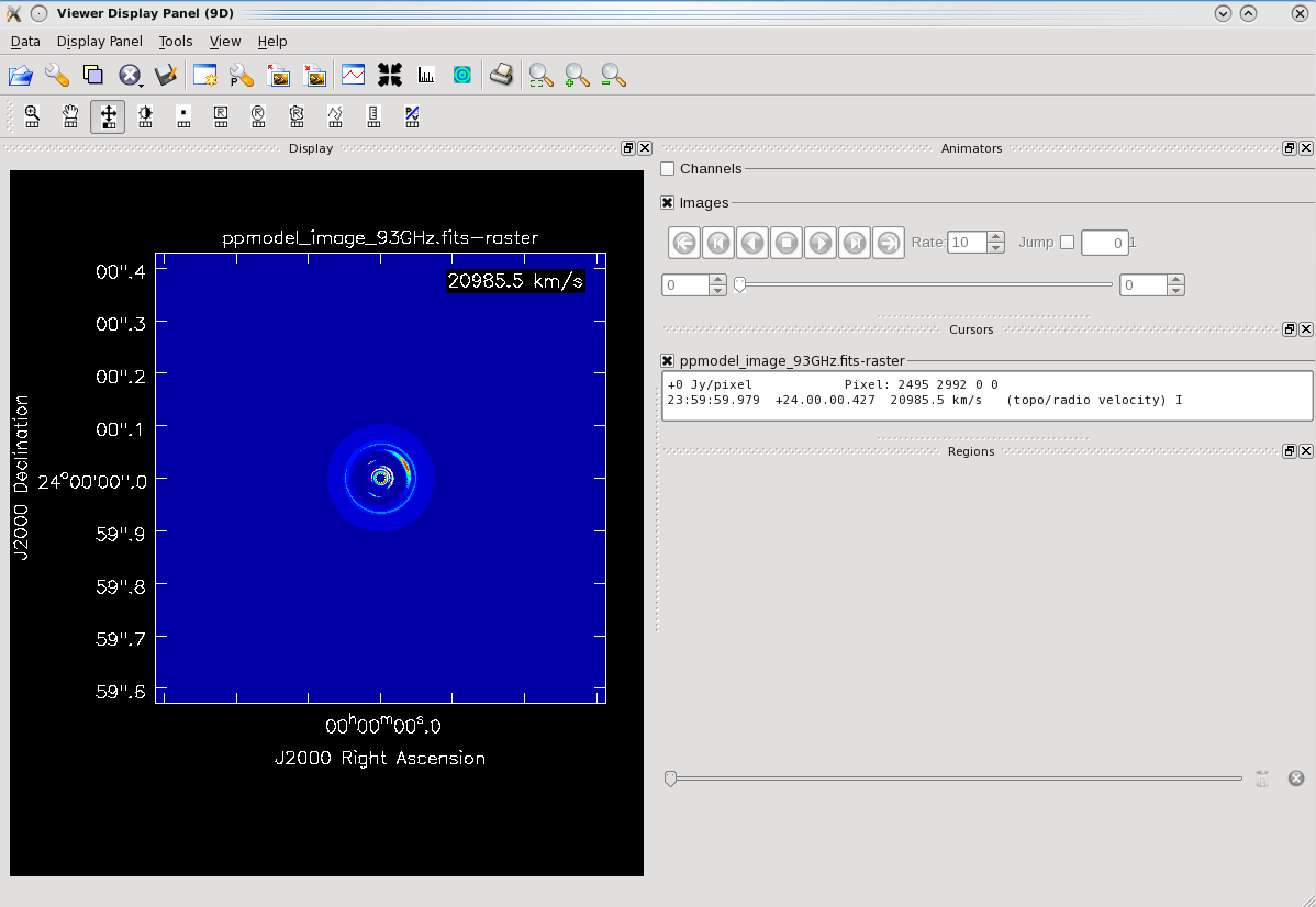
Here we show an example of the resulting images using the resulting simulated MS from Section: "Example simulation using Simobserve with a model image". Fig. 1 shows the model that we use for this simulation tutorial.
 |
Now we will use the simulated MS to make a dirty image. In order to determine an appropriate cell size we use im.advise to find the maximum cell size that will allow the longest baselines to be gridded. We want to avoid using a value larger than this maximum size to ensure that all the data is used during imaging.
# In CASA

im.open('ngVLA_214_ant_60s_noisy.ms')
print( im.advise() )
im.close()
For this MS, im.advise gives a value of 0.0003331 arcseconds which we round down to 0.3 mas . We then choose an image size of 3000 pixels in order to have a field of view comparable to our original model image.
# In CASA

tclean(vis = 'ngVLA_214_ant_60s_noisy.ms', datacolumn = 'data', imagename = 'sm_dirty_noisy', imsize = 3000, cell = '0.3mas',   specmode = 'mfs',  gridder = 'standard', deconvolver = 'hogbom', weighting = 'natural', niter = 0)
We can open the image using the viewer:
# In CASA

viewer('sm_dirty_noisy.image')
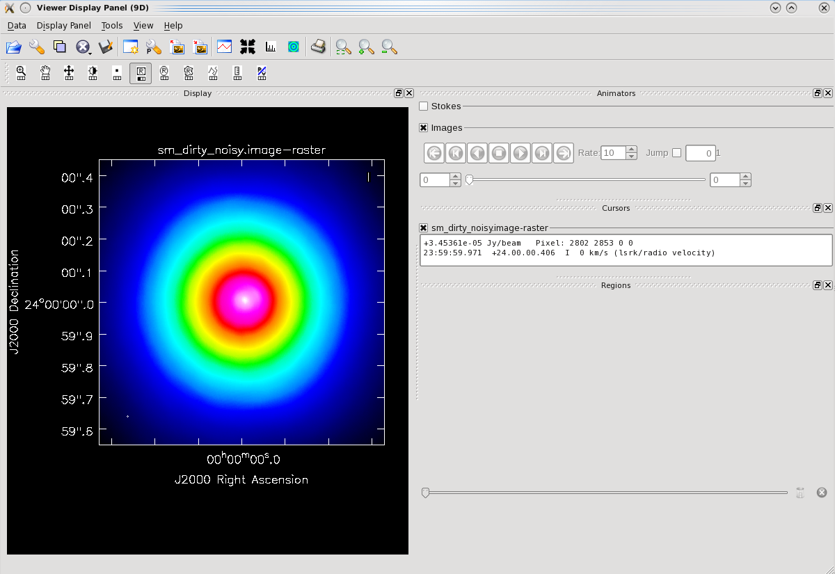
Fig. 2 shows the dirty image.
 |
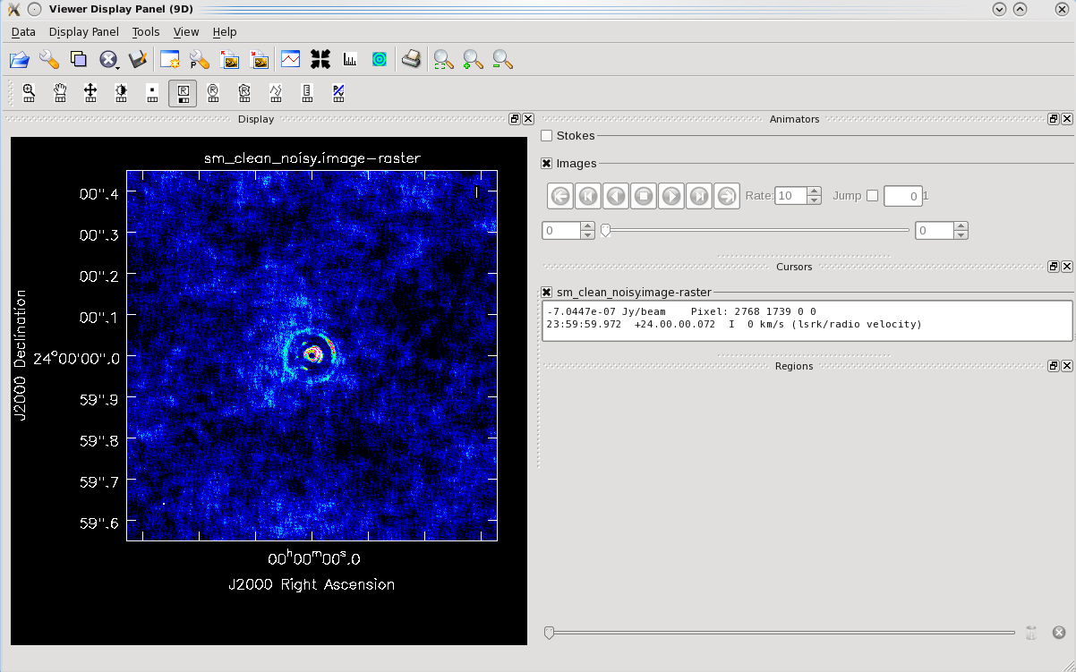
We can also create a perfectly deconvolved image by providing the original model image to the tclean startmodel parameter.
Note: If we tried to clean the dirty image in Fig. 2 instead of using tclean's startmodel parameter, tclean may have had trouble converging to the original model. This can usually be improved by adjusting other imaging parameters (e.g., Briggs weighting, outer UV-taper) at the expense of decreased image sensitivity. These concepts will be explored further in a ngVLA imaging fidelity guide that is currently in preparation.
# In CASA

tclean(vis = 'ngVLA_214_ant_60s_noisy.ms', datacolumn = 'data', imagename = 'sm_clean_noisy', imsize = 3000, cell = '0.3mas',  startmodel = 'ppmodel_image_93GHz.image', specmode = 'mfs',  gridder = 'standard', deconvolver = 'hogbom', weighting = 'natural', niter = 0)
Fig. 3 shows the perfectly deconvolved image. The noise pattern in your image will look different but the magnitude should be similar.
 |
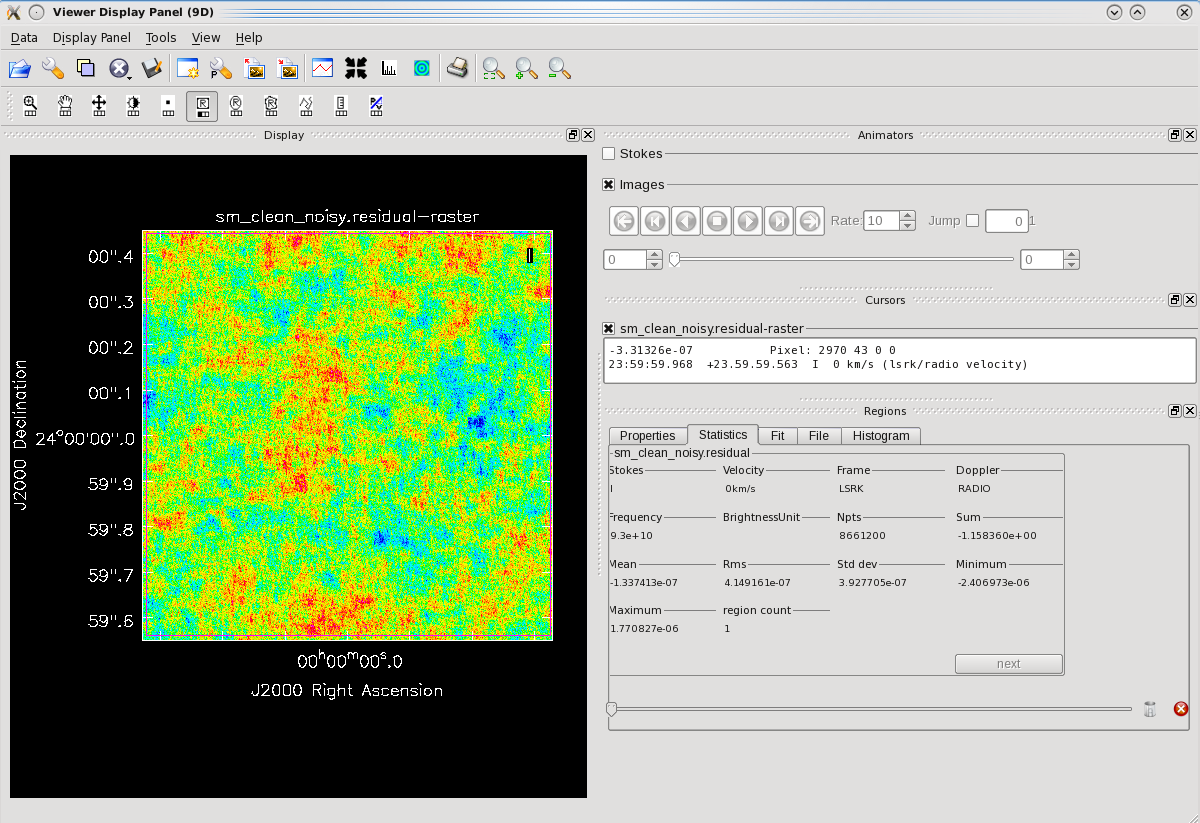
Fig. 4 shows the residual image from the perfect deconvolution. Since the source has been completely deconvolved, the residual image shows the noise that we added with "simplenoise". Using the statistics tab we can see that the image rms and standard deviation are in good agreement with the expected image rms of 0.415 uJy/beam from Section: "Estimating the scaling parameter for adding thermal noise".
 |
Last checked on CASA Version 5.4.1.