Simulating ngVLA Data-CASA5.4.1

tbd simobserve

The following tutorial shows how to simulate next generation very large array (ngVLA) data. The ngVLA is composed of different subarrays that are part of the current reference array. The configuration files are found in "ngVLA Configuration Tools" and can be used for simulations and calculations that investigate the scientific capabilities of the ngVLA. CASA has two simulation tools available: the simobserve task and the sm toolkit. These methods generate measurement sets, add thermal noise and predict model visibilities, from which we can explore the ngVLA’s imaging capabilities. Following we will present three examples: (i) simobserve using a model image, (ii) simobserve using a component list, (iii) sm toolkit simulation. All our examples are at 30 GHz, single channel, 4h integration time, with added thermal noise and no deconvolution. In this example we are going to make a measurement set using the Main ngVLA subarray which is composed of 214 18 m antennas and extends over a maximum baseline of 1005.4 km. The configuration file that we will use through this tutorial is called ngvla-main-revC.cfg and it is found "here".

sm toolkit using either a model image or a component list

# In CASA
## Using the configuration file obtained from the ngVLA's website
conf_file = 'ngvla-main-revC.cfg'
 
## Make an ASCII file with the configuration file i.e., change the extension from .cfg to .tab
tabname = 'antenna_positions_'+conf_file.split('.cfg')[0]+'.tab'     
## The resulting file is called 'antenna_positions_ngvla-main-revC.tab'

## Create a CASA table from an ASCII table using the table utilities (tb) tool
tb.fromascii(tabname, conf_file, firstline=3, sep=' ', columnnames=['X','Y','Z','DIAM','NAME'], datatypes=['D','D','D','D','A'])

xx=[]; yy=[]; zz=[]; 
xx = tb.getcol('X')          ## antenna positions
yy = tb.getcol('Y')
zz = tb.getcol('Z')
diam = tb.getcol('DIAM')     ## diameter of the antennas
anames = tb.getcol('NAME')   ## name of each antenna
tb.close()

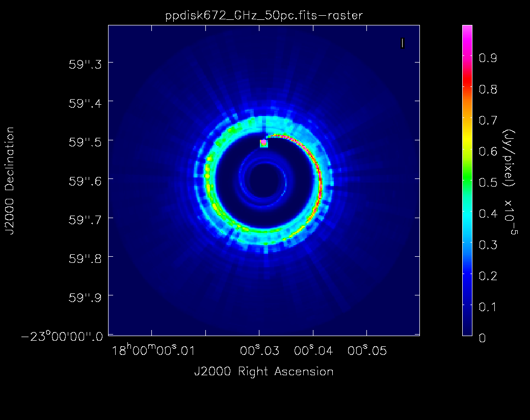
We will use the same image as the ALMA tutorial "Protoplanetary Disk Simulation". Follow this link to obtain the protoplanetary disk model image. Model images are in units of Jy/pixel. Other simulation options, e.g. using component lists, or how to use the toolkit are explained in the Simulations in CASA section of the CASAguides.

Fig. 1 shows the model that we will use for this simulation tutorial.

Fig. 1: Model image of a protoplanetary disk in units of Jy/pixel that we use for this simulation guide.

The ALMA version of the tutorial describes CASA tools to derive the center of the image. We will use their results and specify direction='J2000 18h00m00.031s -22d59m59.6s' for all of our simulations. The image center can also be determined with the CASA viewer. Given that the VLA primary beams at the VLA frequencies are much larger than the image, the precise pointing direction center is less important.

We will mostly use the simobserve and simanalyze tasks similar to the ALMA tutorials (in we will follow the ALMA plotted image sequence). The ALMA model, however, has a specified frequency of 672GHz and we will adapt it to work for VLA frequencies.

Note that simobserve has a few limitations. E.g. it cannot simulate different spectral windows. If this is desired, each spw needs to be simulated separately, followed by a concatenation (concat) of all simulated MeasurementSets. In addition, simobserve has no option to add pointing errors to the simulated data. All VLA configurations and the VLA receiver temperatures are, however, accessible in simobserve.

Q-band, 128MHz bandwidth, noiseless image, 1h integration time, A-configuration, no deconvolution

Let's start with a simulation at 44GHz (Q-band), with a bandwidth of 128MHz, the largest possible bandwidth of a spectral window at the VLA. We will simulate observations with the VLA A-configuration as it provides the resolution that is needed for the disk to be well resolved. To start with, we do not add any noise to the data:

# In CASA
simobserve(project='psimvla1', 
                    skymodel='ppdisk672_GHz_50pc.fits', 
                    inbright='3e-5Jy/pixel', 
                    incenter='44GHz', 
                    inwidth='128MHz' , 
                    setpointings=True, 
                    integration='2s',  
                    direction='J2000 18h00m00.031s -22d59m59.6s',  
                    mapsize= '0.78arcsec', 
                    obsmode='int', 
                    antennalist='vla.a.cfg', 
                    hourangle='transit', 
                    totaltime='3600s',  
                    thermalnoise='', 
                    graphics='both', 
                    overwrite=True)

project: The name of our project is psimvla1. All data will be stored in a directory that is created using the project name.

skymodel: The input model image in Jy/pixel units. We overwrite the fits header to assume that the model is valid for 44GHz with the incenter parameter and the bandwidth to 128MHz with inwidth. We also adjust the peak to a lower [math]\displaystyle{ 3\times10^{-5} }[/math]Jy/pixel value with the inbright parameter, as expected at the lower frequency.

setpointings: allows simobserve to derive the pointing positions by its own algorithm. Given that the primary beam at Q-band is about 1 arcminutes (see the VLA observational status summary (OSS)), and the size of the model is less than an arcsecond, a single pointing will be adequate.

integration: To avoid time smearing, we follow the guidance for data rates in the VLA OSS and assume 2s integration time per visibility.

direction: the center of the map. For a single pointing this is equivalent to the pointing center.

obsmode: int is used for interferometric data such as VLA observations.

antennalist: the VLA configuration antenna position file. The files are available in CASA via 'vla.x.cfg' where 'x' is the name of the array configuration. Here 'vla.a.cfg' is the VLA A configuration (the python command os.getenv("CASAPATH").split()[0]+"/data/alma/simmos/" shows the directory that contains all array configurations that are packaged in CASA)

hourangle: is used to simulate observations at a specific hour angle. We use 'transit' for culmination.

totaltime: This is the time on source.

thermalnoise: We leave this parameter empty for this noise-less simulation.

graphics: 'both' will show graphics on the screen and save them as png files in the project directory.

overwrite: True will overwrite previous results; be careful when running multiple setups as the files may have different names and only the files with the same names will be overwritten.

The output of the simulation is shown in Figs. 2 and 3. The first image is the sky coverage which shows clearly that the primary beam exceeds the size of the model image by far. The other outputs are explained in the caption of Fig. 3.

Last checked on CASA Version 5.4.1.