Protoplanetary Disk Simulation - VLA-CASA5.3.0
The following tutorial shows how to adopt typical parameters for simulating Karl G. Jansky VLA data. We use the same image as the ALMA tutorial Protoplanetary Disk Simulation. Follow this link to obtain the protoplanetary disk model. Models are in units of Jy/pixel. Other simulation options, e.g. using component lists, or how to use the toolkit are available on the Simulations in CASA section of CASAguides.
In Fig. 1 we show the model that we use for this simulation tutorial.
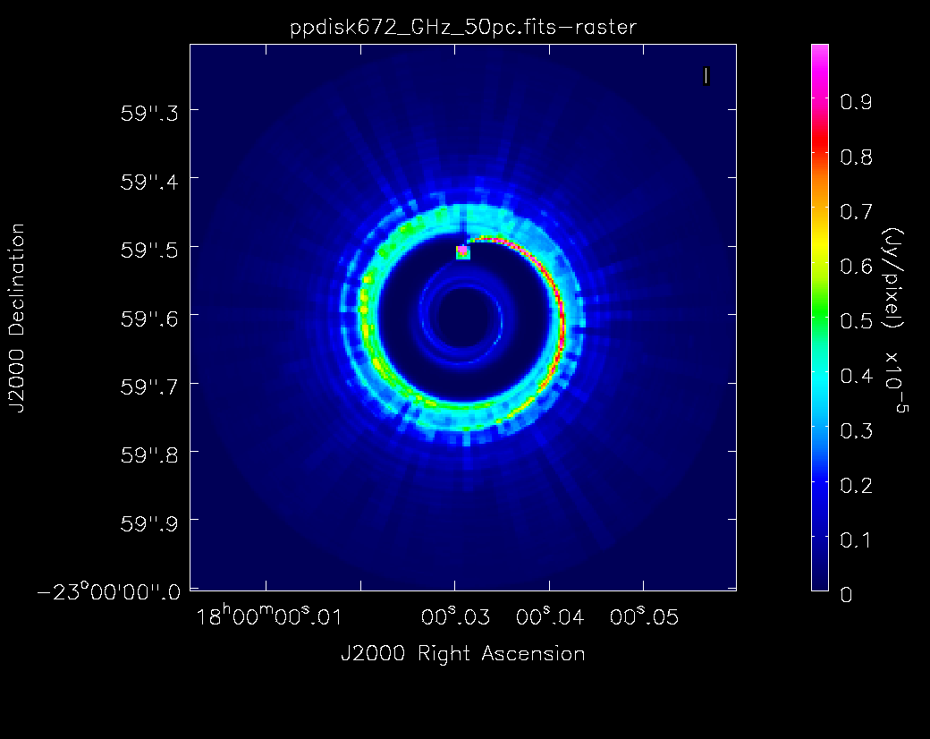 |
The ALMA version of the tutorial shows a way on how to derive the center of the image. We will use their results and specify direction='J2000 18h00m00.031s -22d59m59.6s' for all of our simulations. The image center can also be determined with the CASA viewer. Given that the VLA primary beams at the VLA frequencies are much larger than the image, the precise pointing direction center is less important.
We will use the simobserve and simanalyze tasks as in the ALMA tutorials. The model is derived for 672GHz, we will adapt the simulation to work at VLA frequencies.
Note that simobserve has a few limitations. E.g. it cannot simulate different spectral windows. If this is desired, one needs to set up the simulation for each spw separately, and then use concat to merge all MeasurementSets. simobserve also has no option to add pointing errors to the simulated data. All VLA configurations and the VLA receiver temperatures are, however, accessible in simobserve.
Q-band, 128MHz bandwidth, noiseless image 1h, integration time, no deconvolution
Let's start with a simulation at Q-band at 44GHz, with a bandwidth of 128MHz. We will use the VLA A-configuration as it provides the resolution that is needed for the disk to be well resolved. To start with we do not apply any noise of the data:
# In CASA
simobserve(project='psimvla1', skymodel='ppdisk672_GHz_50pc.fits', inbright='3e-5Jy/pixel', incenter='44GHz', inwidth='128MHz' , setpointings=True, integration='2s',  direction='J2000 18h00m00.031s -22d59m59.6s',  mapsize= '0.78arcsec', obsmode='int', antennalist='vla.a.cfg', hourangle='transit', totaltime='3600s',  thermalnoise='', graphics='both', overwrite=True)
project: The name of our project is psimalma1
skymodel: The input model image in Jy/pixel units. We adjust the peak to a lower $3\times10^{-5}$Jy/pixel value with the inbright parameter. We also overwrite the fits header to assume that the model is valid for 44GHz with incenter and the bandwidth to 128MHz with inwidth
setpointings: will allow simobserve to derive the pointign s by its own algorithm. Given that the primary beam at Q-band is about 1arcminutes (see the VLA [observational status summary], and the size of the model is less than an arcsecond, a single pointing will be more than enough.
integration: To avoid time smearing, we follow the guidance for data rates in the [OSS] and assume 2s per visibility integration.
direction: the center of the map. For a single pointing this is equivalent to the pointing center.
obsmode: int is used for interferometric data such as VLA observations.
antennalist: the VLA configuration antenna position file. The files are available in CASA via 'vla.x.cfg' where 'x' is the name of the array configuration. Here 'vla.a.cfg' is the VLA A configuration (the python command os.getenv("CASAPATH").split()[0]+"/data/alma/simmos/" shows the directory that contains all readily available configurations)
hourangle: is used to simulate observations at a specific hour angle. We use 'transit' for culmination.
totaltime: This is the time on source.
thermalnoise: We leave this parameter empoty for a this noise-less simulation.
graphics: 'both' will show graphics on the screen and save them as png files in the project directory.
overwrite: True will overwrite previous results: be careful when running multiple setups as the files may have different names and only the files with the same names will be overwritten.
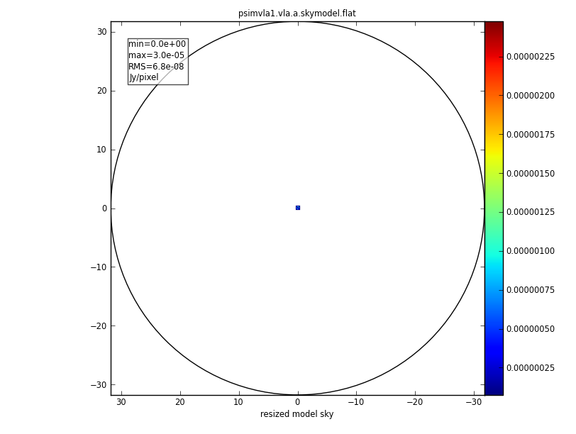
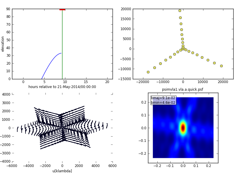
The output of the simulation is shown in Figs. 2 and 3. The first image is the sky coverage which shows clearly that the primary beam exceeds the size of the model image by far.
 |
 |
The task simanalyze can now procvess the nely created MeasurementSet and image the data:
# In CASA
simanalyze(project='psimvla1', image=True, vis='psimvla1.vla.a.ms',  imsize=[192, 192], interactive=False, niter=0, weighting='briggs',  pbcor=True, stokes='I', analyze=True, showuv=False, showpsf=True, showmodel=True, showconvolved=True, showclean=True, showresidual=True, showdifference=True, showfidelity=True, graphics='both', overwrite=True)
project: The project name, same as in our call for simobserve.
image: True will image the visibilities with the following sub-parameters.
vis: The input MeasurementSet. Note that simobserve's notation is to use the project name appended by the antenna configuration file name.
imsize: the number of pixels for the image dimensions. We use 192 for each axis. By default simobserve will use the pixel size of the model image as the cell size for each pixel (3.11 milli-arcseconds in our case).
interactive: If set to True, the cleaning will be interactive to allow the step by step setting of clean boxes and clean depths (see the [VLA imaging topical guide]). We will turn this feature off.
niter: number of clean iterations. We start with a dirty map and set niter=0.
weighting: [Image weighting schemes]. We will use briggs which defaults to a robust = 0.5.
pbcor: If set to True the image will be primary beam corrected. In our case of a very large primary beam (see Fig. 1) primary beam correction will introduce very small corrections.
stokes: The Stokes polarization to be produced, we want Stokes I.
analyze: When set to True simobserve will perform basic analysis of the produced images and produce hard copies of the following displays.
showuv: We set this to False as we already show the uv-coverage in the {simobserve}} output (Fig. 3).
showpsf: Although we already have a plot of that in Fig. 3, we show it here again to have the comparison to the other plots.
showconvolved: produces a plot of the model convolved with the synthesized clean beam.
showclean: shows the deconvolved image (in our case we do not perform deconvolution, but show the plot anyways).
showresidual: a plot of the residual image after deconvolution.
showdifference: displays the difference between output cleaned image and input model sky image convolved with output clean beam, i.e. it shows remaining clean artefacts.
showfidelity: a fidelity image, as defined by $\frac{I}{|I-T|}$ where $I$ is the observed image and $T$ the sky model, see the simanalyze CASAdoc help.
- dirty
# In CASA
simobserve(project='psimvla2', skymodel='ppdisk672_GHz_50pc.fits', inbright='3e-5Jy/pixel', incenter='44GHz', inwidth='128MHz' , setpointings=True, integration='2s',  direction='J2000 18h00m00.031s -22d59m59.6s',  mapsize= '0.78arcsec', obsmode='int', antennalist='vla.a.cfg', hourangle='transit', totaltime='3600s',  thermalnoise='', graphics='both', overwrite=True)
- clean
- In CASA
simanalyze(project='psimvla1', image=True, vis='psimvla1.vla.a.ms', imsize=[192, 192], interactive=False, niter=1000, threshold='1e-4Jy', weighting='briggs', pbcor=True, stokes='I', analyze=True, showuv=False, showpsf=True, showmodel=True, showconvolved=True, showclean=True, showresidual=True, showdifference=True, showfidelity=True, graphics='both', overwrite=True)
- case 2 with pwv 4, 128MHz, 1h observation, A-config.
- In CASA
simobserve(project='psimvla2', skymodel='ppdisk672_GHz_50pc.fits', inbright='3e-5Jy/pixel', incenter='44GHz', inwidth='128MHz' , setpointings=True, integration='2s', direction='J2000 18h00m00.031s -22d59m59.6s', mapsize= '0.78arcsec', obsmode='int', antennalist='vla.a.cfg', hourangle='transit', totaltime='3600s', thermalnoise='tsys-atm', user_pwv=4, t_ground=270.0, graphics='both', overwrite=True)
- In CASA
simanalyze(project='psimvla2', image=True, vis='psimvla2.vla.a.noisy.ms', imsize=[192, 192], interactive=False, niter=1000, threshold='1e-3Jy', weighting='briggs', pbcor=True, stokes='I', analyze=True, showuv=False, showpsf=True, showmodel=True, showconvolved=True, showclean=True, showresidual=True, showdifference=True, showfidelity=True, graphics='both', overwrite=True)
- case 3 extend to 8GHz
- In CASA
simobserve(project='psimvla3', skymodel='ppdisk672_GHz_50pc.fits', inbright='3e-5Jy/pixel', incenter='44GHz', inwidth='8GHz' , setpointings=True, integration='2s', direction='J2000 18h00m00.031s -22d59m59.6s', mapsize= '0.78arcsec', obsmode='int', antennalist='vla.a.cfg', hourangle='transit', totaltime='3600s', thermalnoise='tsys-atm', user_pwv=4, t_ground=270.0, graphics='both', overwrite=True)
- In CASA
simanalyze(project='psimvla3', image=True, vis='psimvla3.vla.a.noisy.ms', imsize=[192, 192], interactive=False, niter=1000, threshold='4e-4Jy', weighting='briggs', pbcor=True, stokes='I', analyze=True, showuv=False, showpsf=True, showmodel=True, showconvolved=True, showclean=True, showresidual=True, showdifference=True, showfidelity=True, graphics='both', overwrite=True)
- case 4 extend to 4h, 8GHz
- In CASA
simobserve(project='psimvla4', skymodel='ppdisk672_GHz_50pc.fits', inbright='3e-5Jy/pixel', incenter='44GHz', inwidth='8GHz' , setpointings=True, integration='2s', direction='J2000 18h00m00.031s -22d59m59.6s', mapsize= '0.78arcsec', obsmode='int', antennalist='vla.a.cfg', hourangle='transit', totaltime='14400s', thermalnoise='tsys-atm', user_pwv=4, t_ground=270.0, graphics='both', overwrite=True)
- In CASA
simanalyze(project='psimvla4', image=True, vis='psimvla4.vla.a.noisy.ms', imsize=[192, 192], interactive=False, niter=1000, threshold='4e-4Jy', weighting='briggs', pbcor=True, stokes='I', analyze=True, showuv=False, showpsf=True, showmodel=True, showconvolved=True, showclean=True, showresidual=True, showdifference=True, showfidelity=True, graphics='both', overwrite=True)
- case 5 then pwv 18mm, 8GHz
- In CASA
simobserve(project='psimvla5', skymodel='ppdisk672_GHz_50pc.fits', inbright='3e-5Jy/pixel', incenter='44GHz', inwidth='8GHz' , setpointings=True, integration='2s', direction='J2000 18h00m00.031s -22d59m59.6s', mapsize= '0.78arcsec', obsmode='int', antennalist='vla.a.cfg', hourangle='transit', totaltime='3600s', thermalnoise='tsys-atm', user_pwv=18, t_ground=270.0, graphics='both', overwrite=True)
- In CASA
simanalyze(project='psimvla5', image=True, vis='psimvla5.vla.a.noisy.ms', imsize=[192, 192], interactive=False, niter=1000, threshold='1e-3Jy', weighting='briggs', pbcor=True, stokes='I', analyze=True, showuv=False, showpsf=True, showmodel=True, showconvolved=True, showclean=True, showresidual=True, showdifference=True, showfidelity=True, graphics='both', overwrite=True)
- case 6 then do C-config. 4mm
- In CASA
simobserve(project='psimvla6', skymodel='ppdisk672_GHz_50pc.fits', inbright='3e-5Jy/pixel', incenter='44GHz', inwidth='8GHz' , setpointings=True, integration='2s', direction='J2000 18h00m00.031s -22d59m59.6s', mapsize= '0.78arcsec', obsmode='int', antennalist='vla.c.cfg', hourangle='transit', totaltime='3600s', thermalnoise='tsys-atm', user_pwv=4, t_ground=270.0, graphics='both', overwrite=True)
- In CASA
simanalyze(project='psimvla6', image=True, vis='psimvla6.vla.c.noisy.ms', imsize=[1728, 1728], interactive=False, niter=1000, threshold='1e-3Jy', weighting='briggs', pbcor=True, stokes='I', analyze=True, showuv=False, showpsf=True, showmodel=True, showconvolved=True, showclean=True, showresidual=True, showdifference=True, showfidelity=True, graphics='both', overwrite=True)
- case 7 then do 4GHz X-band for comparison in a-config
- In CASA
simobserve(project='psimvla7', skymodel='ppdisk672_GHz_50pc.fits', inbright='1e-5Jy/pixel', incenter='10GHz', inwidth='4GHz' , setpointings=True, integration='2s', direction='J2000 18h00m00.031s -22d59m59.6s', mapsize= '0.78arcsec', obsmode='int', antennalist='vla.a.cfg', hourangle='transit', totaltime='3600s', thermalnoise='tsys-atm', user_pwv=4, t_ground=270.0, graphics='both', overwrite=True)
- In CASA
simanalyze(project='psimvla7', image=True, vis='psimvla7.vla.a.noisy.ms', imsize=[192, 192], interactive=False, niter=1000, threshold='1e-3Jy', weighting='briggs', pbcor=True, stokes='I', analyze=True, showuv=False, showpsf=True, showmodel=True, showconvolved=True, showclean=True, showresidual=True, showdifference=True, showfidelity=True, graphics='both', overwrite=True)
==
- pwv 4-18mm
== case 1 simulate data for 43GHz, no noise, 128MHz, 1h observation, A-config.
# In CASA
simobserve(project='psimvla1',   skymodel='ppdisk672_GHz_50pc.fits', inbright='3e-5Jy/pixel', incenter='44GHz', inwidth='128MHz' , setpointings=True, integration='3s',  direction='J2000 18h00m00.031s -22d59m59.6s',  mapsize= '0.78arcsec', obsmode='int', antennalist='vla.a.cfg', hourangle='transit', totaltime='3600s',  thermalnoise='', graphics='both', overwrite=True)
dirty
# In CASA
simanalyze(project='psimvla1', image=True, vis='psimvla.vla.a.ms',  imsize=[192, 192], interactive=False, niter=0, weighting='briggs',  pbcor=True, stokes='I', analyze=True, showuv=False, showpsf=True, showmodel=True, showconvolved=True, showclean=True, showresidual=True, showdifference=True, showfidelity=True, graphics='both', overwrite=True)
clean
# In CASA
simanalyze(project='psimvla1', image=True, vis='psimvla.vla.a.ms',  imsize=[192, 192], interactive=False, niter=1000, threshold='1e-4Jy', weighting='briggs',  pbcor=True, stokes='I', analyze=True, showuv=False, showpsf=True, showmodel=True, showconvolved=True, showclean=True, showresidual=True, showdifference=True, showfidelity=True, graphics='both', overwrite=True)
case 2
with pwv 4, 128MHz, 1h observation, A-config.
# In CASA
simobserve(project='psimvla2', skymodel='ppdisk672_GHz_50pc.fits', inbright='3e-5Jy/pixel', incenter='44GHz', inwidth='128MHz' , setpointings=True, integration='3s',  direction='J2000 18h00m00.031s -22d59m59.6s',  mapsize= '0.78arcsec', obsmode='int', antennalist='vla.a.cfg', hourangle='transit', totaltime='3600s',  thermalnoise='tsys-atm', user_pwv=4, t_ground=270.0, graphics='both', overwrite=True)
# In CASA
simanalyze(project='psimvla2', image=True, vis='psimvla.vla.a.noisy.ms', imsize=[192, 192], interactive=False, niter=1000, threshold='1e-3Jy', weighting='briggs',  pbcor=True, stokes='I', analyze=True, showuv=False, showpsf=True, showmodel=True, showconvolved=True, showclean=True, showresidual=True, showdifference=True, showfidelity=True, graphics='both', overwrite=True)
case 3 extend to 8GHz
# In CASA
simobserve(project='psimvla3',   skymodel=''ppdisk672_GHz_50pc.fits'', inbright='3e-5Jy/pixel', incenter='44GHz', inwidth='8GHz' , setpointings=True, integration='3s',  direction='J2000 18h00m00.031s -22d59m59.6s',  mapsize= '0.78arcsec', obsmode='int', antennalist='vla.a.cfg', hourangle='transit', totaltime='3600s',  thermalnoise='tsys-atm', user_pwv=4, t_ground=270.0, graphics='both', overwrite=True)
# In CASA
simanalyze(project='psimvla3', image=True, vis='psimvla.vla.a.noisy.ms',  imsize=[192, 192], interactive=False, niter=1000, threshold='4e-4Jy', weighting='briggs',  pbcor=True, stokes='I', analyze=True, showuv=False, showpsf=True, showmodel=True, showconvolved=True, showclean=True, showresidual=True, showdifference=True, showfidelity=True, graphics='both', overwrite=True)
case 4
extend to 4h, 8GHz
# In CASA
simobserve(project='psimvla4',   skymodel='ppdisk672_GHz_50pc.fits', inbright='3e-5Jy/pixel',  incenter='44GHz', inwidth='8GHz' , setpointings=True, integration='3s',  direction='J2000 18h00m00.031s -22d59m59.6s',  mapsize= '0.78arcsec', obsmode='int', antennalist='vla.a.cfg', hourangle='transit', totaltime='14400s',  thermalnoise='tsys-atm', user_pwv=4, t_ground=270.0, graphics='both', overwrite=True)
# In CASA
simanalyze(project='psimvla4', image=True, vis='psimvla.vla.a.noisy.ms',  imsize=[192, 192], interactive=False, niter=1000, threshold='4e-4Jy', weighting='briggs',  pbcor=True, stokes='I', analyze=True, showuv=False, showpsf=True, showmodel=True, showconvolved=True, showclean=True, showresidual=True, showdifference=True, showfidelity=True, graphics='both', overwrite=True)
case 5
then pwv 18mm, 8GHz
# In CASA
simobserve(project='psimvla5',   skymodel='ppdisk672_GHz_50pc.fits', inbright='3e-5Jy/pixel',  incenter='44GHz', inwidth='8GHz' , setpointings=True, integration='3s',  direction='J2000 18h00m00.031s -22d59m59.6s',  mapsize= '0.78arcsec', obsmode='int', antennalist='vla.a.cfg', hourangle='transit', totaltime='3600s',  thermalnoise='tsys-atm', user_pwv=18, t_ground=270.0, graphics='both', overwrite=True)
# In CASA
simanalyze(project='psimvla5', image=True, vis='psimvla.vla.a.noisy.ms', imsize=[192, 192], interactive=False, niter=1000, threshold='1e-3Jy', weighting='briggs',  pbcor=True, stokes='I', analyze=True, showuv=False, showpsf=True, showmodel=True, showconvolved=True, showclean=True, showresidual=True, showdifference=True, showfidelity=True, graphics='both', overwrite=True)
case 6 then do C-config. 4mm
# In CASA
simobserve(project='psimvla6',   skymodel='ppdisk672_GHz_50pc.fits', inbright='3e-5Jy/pixel',  incenter='44GHz', inwidth='8GHz' , setpointings=True, integration='3s',  direction='J2000 18h00m00.031s -22d59m59.6s',  mapsize= '0.78arcsec', obsmode='int', antennalist='vla.c.cfg', hourangle='transit', totaltime='3600s',  thermalnoise='tsys-atm', user_pwv=4, t_ground=270.0, graphics='both', overwrite=True)
# In CASA
simanalyze(project='psimvla6', image=True, vis='psimvla.vla.c.noisy.ms',  imsize=[1728, 1728], interactive=False, niter=1000, threshold='1e-3Jy', weighting='briggs',  pbcor=True, stokes='I', analyze=True, showuv=False, showpsf=True, showmodel=True, showconvolved=True, showclean=True, showresidual=True, showdifference=True, showfidelity=True, graphics='both', overwrite=True)
case 7 then do 4GHz X-band for comparison in a-config
# In CASA
simobserve(project='psimvla7',   skymodel='ppdisk672_GHz_50pc.fits', inbright='1e-5Jy/pixel',  incenter='10GHz', inwidth='4GHz' , setpointings=True, integration='3s',  direction='J2000 18h00m00.031s -22d59m59.6s',  mapsize= '0.78arcsec', obsmode='int', antennalist='vla.c.cfg', hourangle='transit', totaltime='3600s',  thermalnoise='tsys-atm', user_pwv=4, t_ground=270.0, graphics='both', overwrite=True)
# In CASA
simanalyze(project='psimvla7', image=True, vis='psimvla.vla.a.noisy.ms',  imsize=[192, 192], interactive=False, niter=1000, threshold='1e-3Jy', weighting='briggs',  pbcor=True, stokes='I', analyze=True, showuv=False, showpsf=True, showmodel=True, showconvolved=True, showclean=True, showresidual=True, showdifference=True, showfidelity=True, graphics='both', overwrite=True)
Protoplanetary Disk Simulation - VLA
- This is an advanced simulation tutorial. New users are recommended to begin with reading the CASA Docs documentation pages on "Simulations".
- This guide is applicable to CASA version 5.1.
- To create a script of the Python code on this page see Extracting scripts from these tutorials.
Data
For this CASA Guide we will use a protoplanetary disk model from S. Wolf. Get the data here. Note that this is a modified image from the ALMA Simulation Inputs, where we changed the center frequency 35GHz and the bandwidth to 128MHz. '
Script with Explanation
Set simobserve as the current task and reset all parameters.
# In CASA
default("simobserve")
Let's call our project "psimvla". This defines the root prefix for any output files from simobserve.
project = "psimvla"
Review the image coordinate system using task imhead.
# This reports image header parameters in the Log Messages window
imhead("ppdisk43_GHz_50pc.fits")
This confirms that the data are set at 43GHz center frequency with a bandwidth of 128MHz. Note that the reference coordinate of the image is at pixel (0,0), i.e. in a corner of the image, not the center. In [[1]] a method is provided on how to derive the image centers through the toolkit. Using that method, or inspecting the image with the viewer shows that the image center is at RA=18h00m00.031s, DEC=-22d59m59.6s.
We'll set skymodel to the FITS file downloaded, above, and leave all skymodel subparameters at their default values. simobserve will create CASA image psimvla.skymodel.
skymodel = "ppdisk43_GHz_50pc.fits"
We will specify the sky position for the center of the observation and set the map size to the size of the model image. The image is very small compared to the VLA primary beam at 35GHz () Since the model image is 2/3 arcseconds across, we should only need one pointing. In this case, pointingspacing and maptype can be left at their default values.
setpointings       =  True
direction          =  "J2000 18h00m00.031s -22d59m59.6s"
mapsize            =  "0.76arcsec"
We do want to simulate an interferometric observation, so we set obsmode accordingly. We'll set totaltime to a 20-minute snapshot observation.
obsmode            =  "int"
totaltime          =  "1200s"
We want to use the appropriate antenna configuration for the desired angular resolution. Configuration 20, alma.out20.cfg, is the largest "compact" configuration. A list of configuration files available in CASA 4.1 is available here.
antennalist = "vla.a.cfg"
We do not want to simulate observations with thermal noise in this example, so we set:
thermalnoise = ''
Now run simobserve.
simobserve()
Now that we've simulated the visibility measurements, we want to generate an image from the simulated data. simanalyze makes this easy. We begin by setting project to the same prefix used in simobserve and setting image to True.
default ("simanalyze")
project = "psimvla"
image = True
We set modelimage to use the input FITS image when cleaning the simulated visibilities. We set the image size to 192 pixels square.
modelimage = "ppdisk43_GHz_50pc.fits"
vis = project + ".vla.a.ms"
imsize = [192, 192]
Specify the number of iterations for cleaning, with proper threshold and weighting.
niter = 10000
threshold = "1e-7Jy"
weighting = "natural"
We'd like to calculate a difference and fidelity image, but we don't need to see the uv coverage.
analyze = True
showuv = False
showresidual = True
showconvolved = True
Plot both to the screen and PNG files with lots of messages.
graphics = "both"
verbose = True
overwrite = True
Run simanalyze.
simanalyze()
Simulation Output
Input: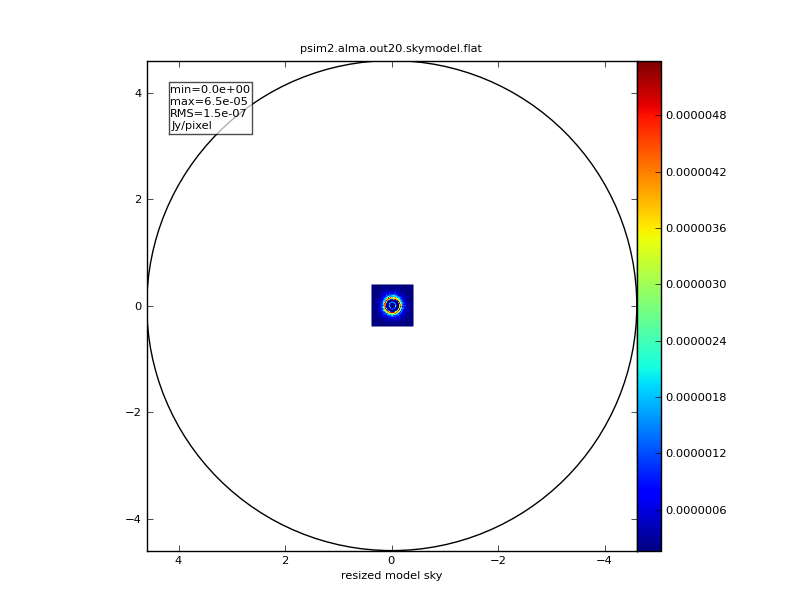
|
simobserve: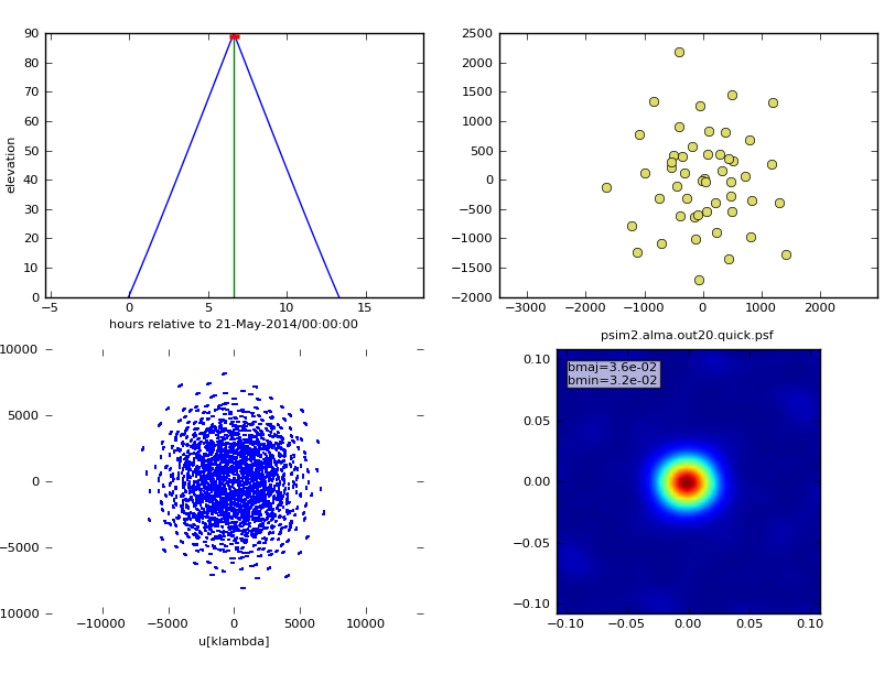
|
simanalyze image: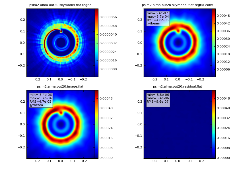
|
simanalyze output: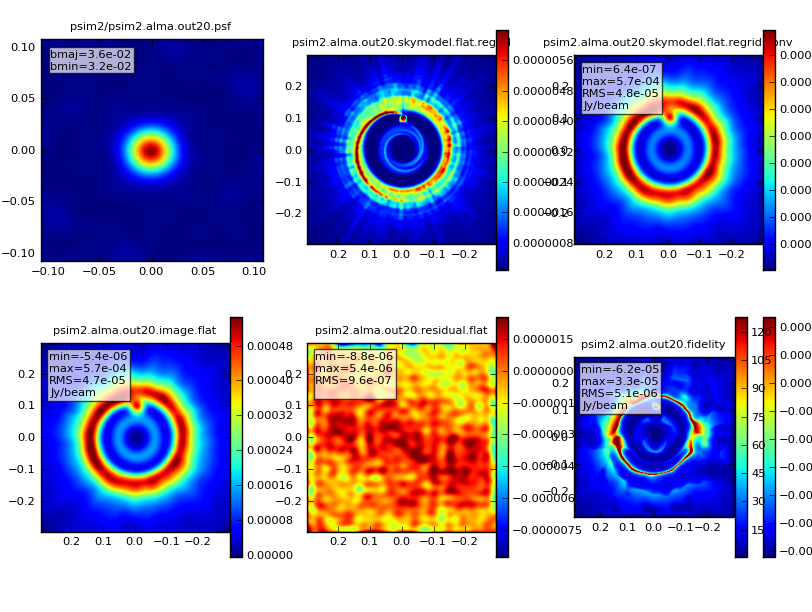
|