Imaging Prep
Imaging Prep Workflow
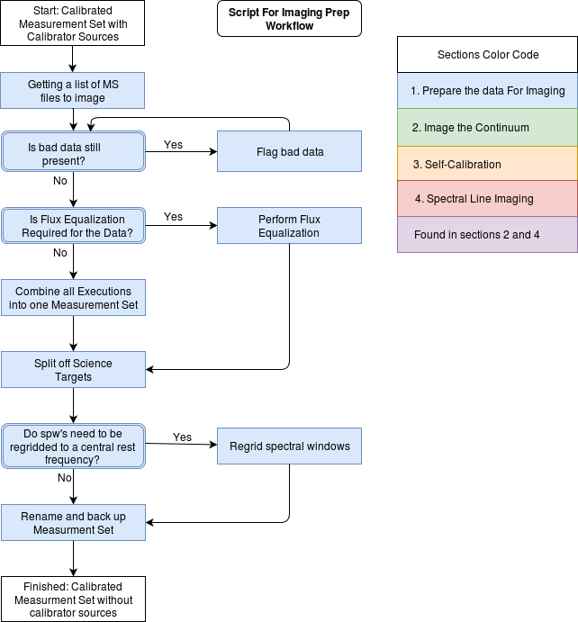
Use the Imaging Prep workflow to determine which sections of this guide are applicable to your dataset.
Get a list of ms files to image
<figure id="Weblog_Home.png">
</figure> Once the calibration has run, it will produce ‘*.ms.split.cal’ files for each execution. These files contain the calibrated data. Run the following commands to grab the names of all files in the directory that have the extension ‘.ms.split.cal’ and place them into a list.
# in CASA
import glob
vislist=glob.glob('*.ms.split.cal')
Review the Calibration
Once the list of measurement set (ms) files have been collected, review the calibration to make sure it appears reasonable. A summary of the calibration are in the qa directory of your delivered package. If the dataset was pipeline calibrated, download and untar the pipeline file in the qa directory by using <figure id="Weblog_MS_Overview.png">
</figure>
# in bash
for i in $(ls *.tar); do tar -xvf $i; done
# or in CASA
For i in glob.glob(‘*.tar’):
	os.system(‘tar -xvf %s’ % (i))
Once this is done, look within the /html directory for the index.html file. This contains the html code for displaying the contents of the qa directory in a web browser. The command below opens the main page of the weblog in firefox.
firefox index.html
<figure id="Weblog_By_Task.png">
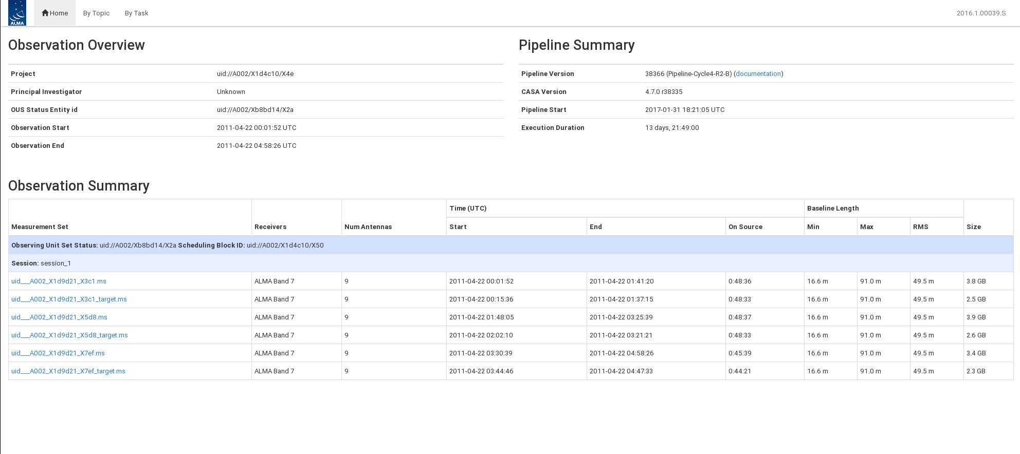
</figure> The standard opening page has three main sections: observation overview, pipeline summary, and observation summary. This is shown in Figure 1.
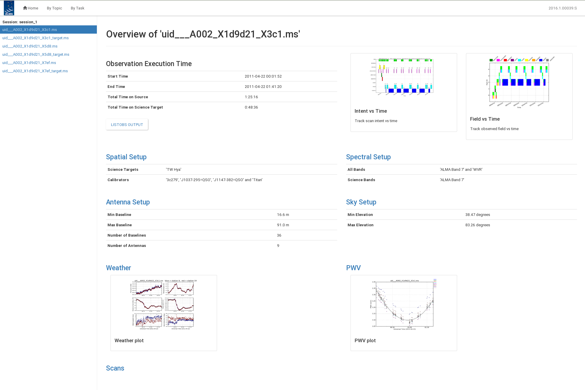
From the opening page, you can navigate to view the calibration By Topic and By Task and open observation specific information by clicking on the ms name. Figure 2 shows an example of an ms summary page.
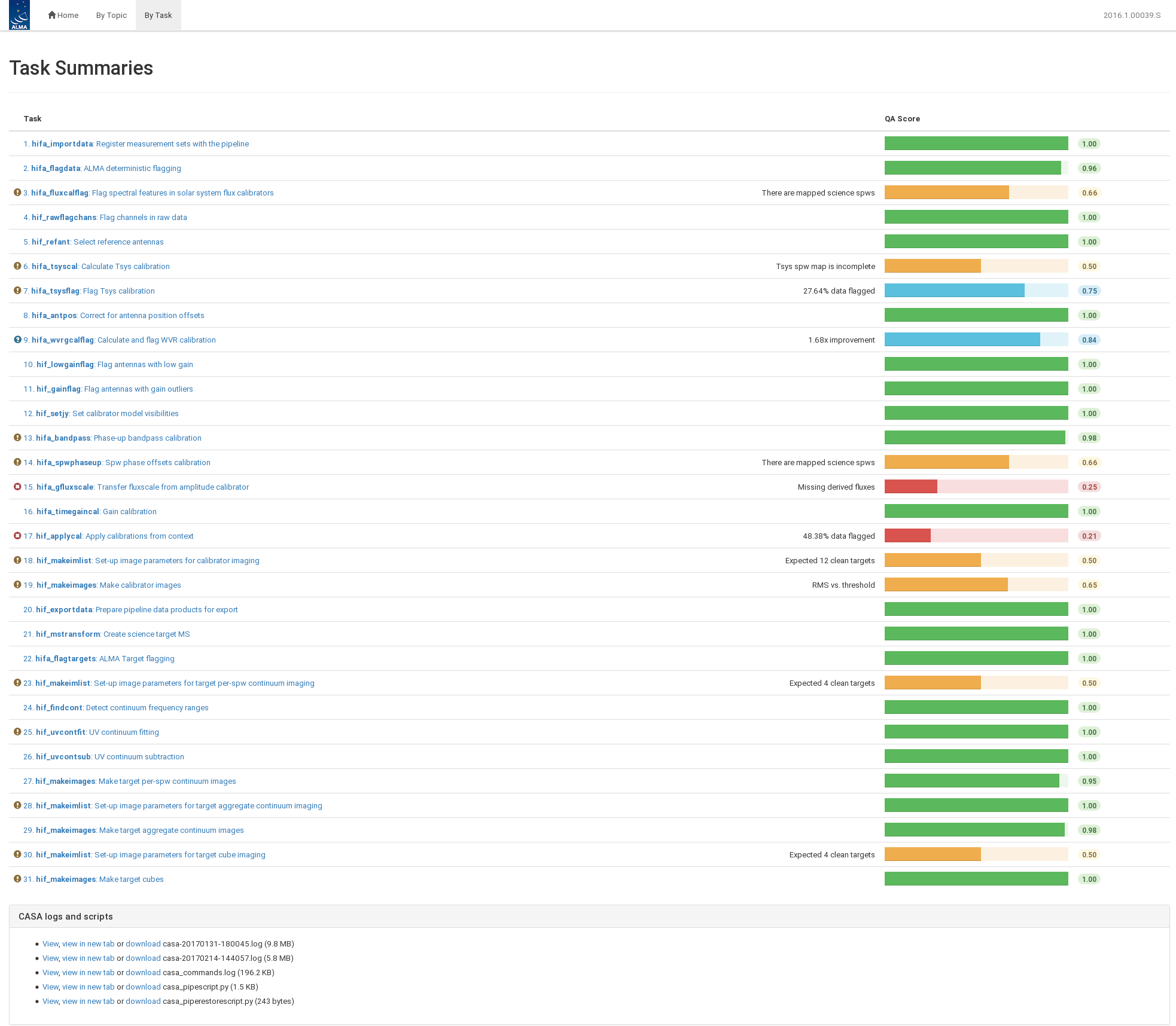
Figure 3 shows the By Task view. Each task can be opened to view important calibration plots, tables, and flagging statistics.
If the data was manually calibrated, you can review the calibration with the *.png and *.txt files in the qa directory. These display helpful plots and statistics about the calibration.
In addition, the tasks plotms and plotcal are useful if you need to explore the data beyond the plots that the calibration pipeline or QA2 process generates. The TW Hydra guide gives some nice examples showing how to use these tasks.
Flag bad data (optional)
Save the original flags of each ms prior to flagging any additional data. Without this step, it will be very difficult if you need to remove flags generated later on.
# in CASA
for vis in vislist:
    flagmanager(vis=vis,
                mode='save',
                versionname='original_flags')
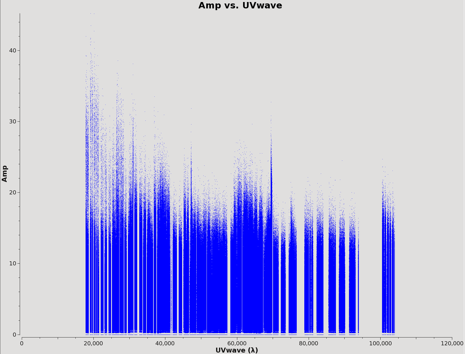
The plotms task can be used to find bad data by iterating through fields and spws for the *.ms.split.cal files in the calibrated directory. You can also use the GUI interface to iterate through spectral windows (spws). Figure 4 shows an example of TW Hydra science spw 2.
# in CASA
fieldlist = ['3'] # change to list of science data fields to inspect
spwlist = ['1'] # change to list of science spws to inspect

for vis in vislist:
    for field in fieldlist:
        for spw in spwlist:
            plotms(vis=vis,xaxis='uvwave',yaxis='amp',avgtime='3e8',
                   field=field,spw=spw)
            raw_input("push enter to continue")
            plotms(vis=vis,xaxis='chan',yaxis='amp',avgtime='3e8',
                   field=field,spw=spw)
            raw_input("push enter to continue")
Use flagdata to flag bad antennas, spws, timeranges, etc. You can use the locate buttons in plotms and plotcal to identify what needs to be flagged. Note that flagging in plotms is generally not recommended because a plotms crash will lose all flagging information.
To flag data, modify the following command with the specific ms name with the vis parameter and any antenna, spw, etc. Once the data is flagged, check the flagging using plotms. The flagged data points should not appear on the plot. You can also plot the flagged data points using the "display" table on the left hand side of the plotms GUI. <figure id="TWHydra_corrected_Spw2.png">
</figure>
# in CASA
flagdata(vis='',mode='manual',action='apply',flagbackup=False)
If you need to restore original flags, use the following command. You will need to update the ms name in the vis parameter.
# in CASA
flagmanager(vis='',mode='restore',versionname='original_flags')
Flux Equalization (optional)
If you have multiple executions taken at a similar time with the same phase calibrator, you can rescale the derived fluxes for the phase calibrator so that they are the same in all executions. If the executions are spaced by more than a day or two, it is likely the flux of the phase calibrator has changed and thus this step is usually unnecessary. You can compared the derived flux densities of your calibrators for each execution block using the "hifa_gfluxscale" step of the weblog (pipeline calibrations) or the *.fluxscale file (manual calibration).
The following guides may be useful for assessing the derived fluxes of your phase cailbrators. ALMA Memo 434 outlines various uncertainties relevant to amplitude calibration. You can refer to the respective cycle’s Proposer’s Guide (Cycle 4) for expected uncertainties. In addition, the ALMA Calibrator Source Catalog can be used to compare variations detected from source monitoring.
<figure id="Gfluxscale table.png">

</figure>
If you have determined flux equalization is required for your data, please file a Helpdesk ticket (help.almascience.org) and a NAASC staff member can assist you by generating a script for your measurement sets. In general, the first step in flux equalization is setting the flux density of the phase calibrator in each spectral window to the desired value using setjy. Then amplitude calibration tables are generated and applied using gaincal and applycal respectively. Finally, all calibrated measurement sets will be concatenated using concat.
If you have performed flux equalization, you can skip to the Splitting off science target data section below.
Combining measurement sets from multiple executions
If there are multiple *.ms.split.cal files within the calibrated directory, you will want to combine them all into one single ms file in order to make later steps in the imaging process easier. Skip this section if you have only one execution.
Each execution of the scheduling block will generate multiple spectral windows with different sky frequencies, but the same rest frequency, due to the motion of the Earth. Thus, the resulting concatenated file will contain n spws, where n is (number of original science spws) x (number of executions). In other words, the multiple spws associated with a single rest frequency will not be regridded to a single spectral window in the ms. Combine all executions into one ms file, called calibrated.ms, using the concat command.
# in CASA
concatvis='calibrated.ms'

rmtables(concatvis)
os.system('rm -rf ' + concatvis + '.flagversions')
concat(vis=vislist,
   concatvis=concatvis)
Splitting off science target data
The calibrated.ms produced in the Combining measurement sets from multiple executions section, or your original ms file if you only have one execution, will contain the science target(s) as well as all the calibrator sources. At this point, you are only concerned with imaging your science targets so you can split them off from the calibrated.ms which has both the science and calibrator sources. This will reduce the size of the file and make it more manageable during imaging. Depending on your project, there may be several executions or only one. Uncomment the line that fits with your data to set the concatvis variable properly.
# in CASA
# Uncomment following line for single executions
# concatvis = vislist[0]

# Uncomment following line for multiple executions
# concatvis='calibrated.ms'
You will split out all target fields from the file and copy them, with only the data column, into a new ms file called calibrated_source.ms. Follow this link for more information regarding the structure of measurement sets.
# in CASA
sourcevis='calibrated_source.ms'
rmtables(sourcevis)
os.system('rm -rf ' + sourcevis + '.flagversions')
split(vis=concatvis,
  intent='*TARGET*', # split off the target sources
  outputvis=sourcevis,
  datacolumn='data')
At this point, it is convenient to create a listobs file with information about the sources and spectral windows to reference during imaging. Inspect the listobs to make sure the split and concat worked as desired.
# in CASA
listobs(vis=sourcevis,listfile=sourcevis+'.listobs.txt')
An example listobs file is below.
================================================================================
   Observer: Unknown     Project: T.B.D.
Observation: ALMA

  Telescope Observation Date    Observer       Project
  ALMA      [                   4.81015e+09, 4.81015e+09]Unknown        T.B.D.
  ALMA      [                   4.81015e+09, 4.81016e+09]Unknown        T.B.D.
  ALMA      [                   4.81016e+09, 4.81017e+09]Unknown        T.B.D.
Data records: 126900       Total elapsed time = 16902.1 seconds
   Observed from   22-Apr-2011/00:15:36.7   to   22-Apr-2011/04:57:18.8 (UTC)

   ObservationID = 0         ArrayID = 0
  Date        Timerange (UTC)          Scan  FldId FieldName             nRows     SpwIds   Average Interval(s)    ScanIntent
  22-Apr-2011/00:15:36.7 - 00:16:07.0     9      0 TW Hya                     540  [0,1,2,3]  [10.1, 10.1, 10.1, 10.1] [OBSERVE_TARGET#ON_SOURCE]
              00:20:57.8 - 00:30:43.2    13      0 TW Hya                    8640  [0,1,2,3]  [10.1, 10.1, 10.1, 10.1] [OBSERVE_TARGET#ON_SOURCE]
              00:36:49.2 - 00:44:43.5    18      0 TW Hya                    7020  [0,1,2,3]  [10.1, 10.1, 10.1, 10.1] [OBSERVE_TARGET#ON_SOURCE]
              00:49:33.9 - 00:59:19.3    22      0 TW Hya                    8640  [0,1,2,3]  [10.1, 10.1, 10.1, 10.1] [OBSERVE_TARGET#ON_SOURCE]
              01:05:46.8 - 01:13:41.2    27      0 TW Hya                    7020  [0,1,2,3]  [10.1, 10.1, 10.1, 10.1] [OBSERVE_TARGET#ON_SOURCE]
              01:20:07.2 - 01:29:52.6    31      0 TW Hya                    8640  [0,1,2,3]  [10.1, 10.1, 10.1, 10.1] [OBSERVE_TARGET#ON_SOURCE]
              01:37:15.6 - 01:40:13.9    36      0 TW Hya                    2700  [0,1,2,3]  [10.1, 10.1, 10.1, 10.1] [OBSERVE_TARGET#ON_SOURCE]

   ObservationID = 1         ArrayID = 0
  Date        Timerange (UTC)          Scan  FldId FieldName             nRows     SpwIds   Average Interval(s)    ScanIntent
  22-Apr-2011/02:02:10.9 - 02:02:41.1    44      0 TW Hya                     540  [0,1,2,3]  [10.1, 10.1, 10.1, 10.1] [OBSERVE_TARGET#ON_SOURCE]
              02:07:36.7 - 02:17:22.0    48      0 TW Hya                    8640  [0,1,2,3]  [10.1, 10.1, 10.1, 10.1] [OBSERVE_TARGET#ON_SOURCE]
              02:23:35.7 - 02:31:30.0    53      0 TW Hya                    7020  [0,1,2,3]  [10.1, 10.1, 10.1, 10.1] [OBSERVE_TARGET#ON_SOURCE]
              02:36:23.6 - 02:46:09.0    57      0 TW Hya                    8640  [0,1,2,3]  [10.1, 10.1, 10.1, 10.1] [OBSERVE_TARGET#ON_SOURCE]
              02:52:40.2 - 03:00:34.6    62      0 TW Hya                    7020  [0,1,2,3]  [10.1, 10.1, 10.1, 10.1] [OBSERVE_TARGET#ON_SOURCE]
              03:05:14.0 - 03:14:59.4    66      0 TW Hya                    8640  [0,1,2,3]  [10.1, 10.1, 10.1, 10.1] [OBSERVE_TARGET#ON_SOURCE]
              03:21:21.4 - 03:24:19.6    71      0 TW Hya                    2700  [0,1,2,3]  [10.1, 10.1, 10.1, 10.1] [OBSERVE_TARGET#ON_SOURCE]

   ObservationID = 2         ArrayID = 0
  Date        Timerange (UTC)          Scan  FldId FieldName             nRows     SpwIds   Average Interval(s)    ScanIntent
  22-Apr-2011/03:44:46.9 - 03:45:17.1    79      0 TW Hya                     540  [0,1,2,3]  [10.1, 10.1, 10.1, 10.1] [OBSERVE_TARGET#ON_SOURCE]
              03:50:08.4 - 03:59:53.7    83      0 TW Hya                    8640  [0,1,2,3]  [10.1, 10.1, 10.1, 10.1] [OBSERVE_TARGET#ON_SOURCE]
              04:06:03.7 - 04:13:58.1    88      0 TW Hya                    7020  [0,1,2,3]  [10.1, 10.1, 10.1, 10.1] [OBSERVE_TARGET#ON_SOURCE]
              04:18:49.1 - 04:28:34.4    92      0 TW Hya                    8640  [0,1,2,3]  [10.1, 10.1, 10.1, 10.1] [OBSERVE_TARGET#ON_SOURCE]
              04:34:59.5 - 04:42:53.9    97      0 TW Hya                    7020  [0,1,2,3]  [10.1, 10.1, 10.1, 10.1] [OBSERVE_TARGET#ON_SOURCE]
              04:47:33.5 - 04:57:18.8   101      0 TW Hya                    8640  [0,1,2,3]  [10.1, 10.1, 10.1, 10.1] [OBSERVE_TARGET#ON_SOURCE]
           (nRows = Total number of rows per scan)
Fields: 1
  ID   Code Name                RA               Decl           Epoch   SrcId      nRows
  0    none TW Hya              11:01:51.844983 -34.42.17.16088 J2000   0         126900
Spectral Windows:  (4 unique spectral windows and 1 unique polarization setups)
  SpwID  Name   #Chans   Frame   Ch0(MHz)  ChanWid(kHz)  TotBW(kHz) CtrFreq(MHz)  Corrs
  0              3840   TOPO  356497.936       122.070    468750.0 356732.2500   XX  YY
  1              3840   TOPO  357734.314       122.070    468750.0 357968.6279   XX  YY
  2              3840   TOPO  346034.314       122.070    468750.0 345800.0000   XX  YY
  3              3840   TOPO  343955.936       122.070    468750.0 343721.6221   XX  YY
Sources: 4
  ID   Name                SpwId RestFreq(MHz)  SysVel(km/s)
  0    TW Hya              0     -              -
  0    TW Hya              1     -              -
  0    TW Hya              2     -              -
  0    TW Hya              3     -              -
Antennas: 9:
  ID   Name  Station   Diam.    Long.         Lat.                Offset from array center (m)                ITRF Geocentric coordinates (m)
                                                                     East         North     Elevation               x               y               z
  0    DV04  J505      12.0 m   -067.45.18.0  -22.53.22.8         -7.2141     -541.3485       15.0178  2225061.036842 -5440128.036234 -2481534.422455
  1    DV06  T704      12.0 m   -067.45.16.2  -22.53.22.1         42.8987     -520.1911       15.0694  2225110.551677 -5440116.726350 -2481514.951072
  2    DV07  J510      12.0 m   -067.45.17.8  -22.53.23.5         -0.3652     -563.8032       14.9605  2225064.049398 -5440117.310745 -2481555.086720
  3    DV08  T703      12.0 m   -067.45.16.2  -22.53.23.9         42.8798     -575.6928       14.6278  2225102.207484 -5440096.375809 -2481565.910698
  4    DV09  N602      12.0 m   -067.45.17.4  -22.53.22.3          8.8012     -527.8598       15.0513  2225077.857538 -5440126.858119 -2481522.008896
  5    DV10  N606      12.0 m   -067.45.17.1  -22.53.23.6         19.1981     -566.5667       14.9520  2225081.746122 -5440108.902762 -2481557.629365
  6    PM01  T702      12.0 m   -067.45.18.6  -22.53.24.1        -23.6269     -582.3103       14.9195  2225039.780230 -5440119.418780 -2481572.120530
  7    PM02  T701      12.0 m   -067.45.18.8  -22.53.22.2        -29.1268     -522.7917       15.0566  2225043.501617 -5440143.045000 -2481517.341976
  8    PM03  J504      12.0 m   -067.45.17.0  -22.53.23.0         22.2015     -550.2548       14.9948  2225086.942689 -5440113.674706 -2481542.618537
Regridding spectral window (optional)
ALMA does what is called doppler setting, which means it adjusts the observed sky frequency for the motion of the source and the motion of the Earth around the Sun at the beginning of every execution block. Therefore, different execution blocks will have different observed sky frequencies because the vector of the motion of the Earth around the Sun will be different at different times.
In general, we strongly recommend using the clean command to regrid spectral windows to a common velocity/rest frequency scale on the fly. However, you may also regrid the frequency axis of the visibility data using cvel prior to imaging. The most common use case for this is where the motion of the Earth around the Sun causes the sky frequencies of the lines to shift too much between executions to identify a common channel range for continuum subtraction. If you regrid using cvel prior to imaging, you should make sure to use the same input parameters to the tclean task that you used for cvel. In other words, you shouldn't regrid the data using both cvel and clean.
Due to a bug in all released versions of CASA, mstransform and cvel should not be used to average greater than 2 channels together. This averaging should be done using clean until the bug is resolved.
We will start by setting the parameters specific to your observations.
# in CASA
sourcevis='calibrated_source.ms'
regridvis='calibrated_source_regrid.ms'
veltype = 'radio' # Keep set to radio. See notes in imaging section.
width = '0.23km/s' # due to bug in cvel/mstransform, do not regrid > 2 channels
nchan = -1 # leave this as the default
mode='velocity' # see science goals in the OT
start='' # leave this as the default
outframe = 'bary' # velocity reference frame. see science goals in the OT.
restfreq='115.27120GHz' # rest frequency of primary line of interest.
 field = '4' # select science fields.
spw = '0,5,10' # spws associated with a single rest frequency. Do not attempt to combine spectral windows associated with different rest frequencies. This will take a long time to regrid and most likely isn't what you want.
Regridding here uses the cvel command to regrid multiple spws associated with a single rest frequency into a single spw. To avoid clean regridding the image a second time you will need to use the same parameters used for cvel for clean.
# in CASA
rmtables(regridvis)
os.system('rm -rf ' + regridvis + '.flagversions')

cvel(vis=sourcevis,
     field=field,
     outputvis=regridvis,
     spw=spw,
     mode=mode,
     nchan=nchan,
     width=width,
     start=start,
     restfreq=restfreq,
     outframe=outframe,
     veltype=veltype)
Rename and backup data set
Depending on the different tasks that were performed above, the current measurement set will have a variety of names. For ease of beginning imaging with a common measurement set, rename the file to calibrated_final.ms.
If you haven’t regridded, your current ms should be named calibrated_source.ms.
# in CASA
# uncomment if you haven’t regridded
# os.system('mv -i ' + sourcevis + ' ' + 'calibrated_final.ms')
If you have regridded, your current ms should be named calibrated_source_regrid.ms.
# in CASA
# uncomment if you have regridded
# os.system('mv -i ' + regridvis + ' ' + 'calibrated_final.ms')
Now that you have fully calibrated measurement set containing all your science sources to image, we recommend creating a backup of the dataset. It is possible to corrupt a measurement set if you kill clean, tclean, and uvcontsub while they are running.
# in CASA
os.system('cp -ir calibrated_final.ms calibrated_final.ms.backup')
Continue to Imaging
This guide is continued at Image the Continuum Template.