TWHydraBand7 Imaging 4.5
- This tutorial picks up where TWHydraBand7_Calibration_4.5 leaves off, with fully calibrated, split science target MS. If you wish to skip the Calibration guide: obtain the calibrated data from TWHydraBand7#Getting_the_Data; extract it using tar -xzvf FILENAME; and cd into the extracted directory.
- This guide is designed for CASA 4.5.2. If you are using an older version of CASA please see TWHydraBand7_Imaging_4.3.
- Details of the ALMA data are provided at TWHydraBand7
Confirm your version of CASA
This guide has been written for CASA release 4.5.2. Please confirm your version before proceeding.
# In CASA
version = casadef.casa_version
print "You are using " + version
if (version < '4.5.0'):
    print "YOUR VERSION OF CASA IS TOO OLD FOR THIS GUIDE."
    print "PLEASE UPDATE IT BEFORE PROCEEDING."
else:
    print "Your version of CASA is appropriate for this guide."
Prepare Continuum Data for Further Processing
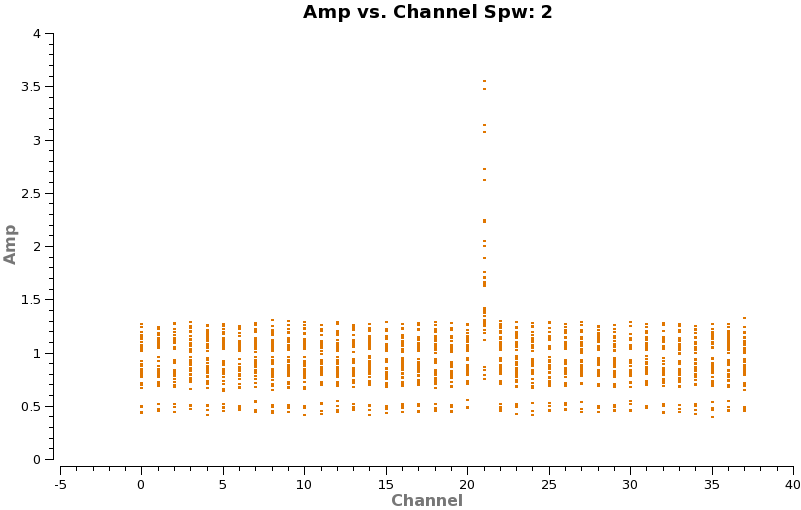
In order to speed up imaging/self-calibration for the continuum data we will average channels together, and then flag the few spectral features. This method works well in the case of only a few spectral lines, while retaining enough channelization to aid in multi-frequency synthesis and being able to remove spectral features in the averaged data. When generalizing this process to other datasets, the amount of channel averaging will vary. Note for wide bandwidth data it is never a good idea to use the continuum estimate generated by uv-continuum subtraction as your continuum data. This worked OK in the past with the narrow band systems like the VLA and low dynamic range instruments like the SMA, but is not advised for ALMA wide bandwidth, high dynamic range data.
<figure id="Cont_spw2.png">
</figure> <figure id="Cont_spw3.png">
</figure>
One can also flag the spectral features first but in that case make a backup of the file that is analogous to TWHydra_corrected.ms as you will need it later (unflagged) for spectral line imaging. We begin by excluding ~20 channels on each edge, and averaging over 100 channel intervals:
# In CASA
os.system('rm -rf TWHydra_cont.ms*')
split(vis='TWHydra_corrected.ms',outputvis='TWHydra_cont.ms',
       spw='0~3:21~3820',width=100,datacolumn='data')
Now make a plot of amplitude vs. channel to see what needs to be flagged
# In CASA
plotms(vis='TWHydra_cont.ms',spw='0~3',xaxis='channel',yaxis='amp',
      avgtime='1e8',avgscan=True,coloraxis='spw',iteraxis='spw',xselfscale=True)
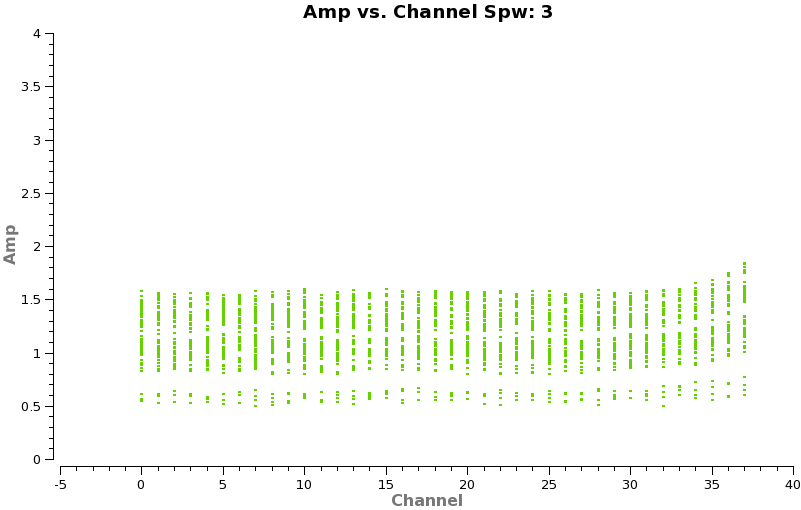
The CO(3-2) and HCO+(4-3) lines are obvious. The 4th spw; spw=3 also shows an upswing on the highest channels that is problematic, it was seen on the calibrators too and is likely due to a weak atmospheric feature, we will flag the worst of it.
<figure id="Cont_uvplot.png">
</figure>
# In CASA
flagdata(vis='TWHydra_cont.ms', mode='manual',
         spw='0:16~16, 2:21~21, 3:33~37')
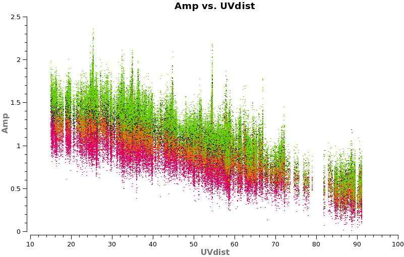
Have a look at the continuum as a function of uv-distance (in the plot to the right, the 4 spw are shown in different colors on top of each other). If the data are flat as a function of uv-distance, the source is completely unresolved. If instead you see structure (in this case decreasing amplitude with uv-distance), the source is resolved.
# In CASA
plotms(vis='TWHydra_cont.ms',spw='',xaxis='uvdist',yaxis='amp',field='',avgchannel='38',
       coloraxis='spw',plotfile='cont_uvplot.png')
Notice that the spw do not have the same amplitude. Unfortunately, the red spw (highest frequency) should be higher than the green one (lowest frequency) because optically thin dust goes as nu^4, and optically thick as nu^2. This inconsistency is due to imperfect amplitude/absolute flux calibration. The self-calibration below will bring them into agreement with each other, but this is the sort of thing that results in considerable absolute flux uncertainty at submillimeter wavelengths. We are working on how to do this better.
A priori Noise Estimates
<figure id="Corrected_time.png">
</figure> <figure id="sensitivity_cont.png">
</figure>
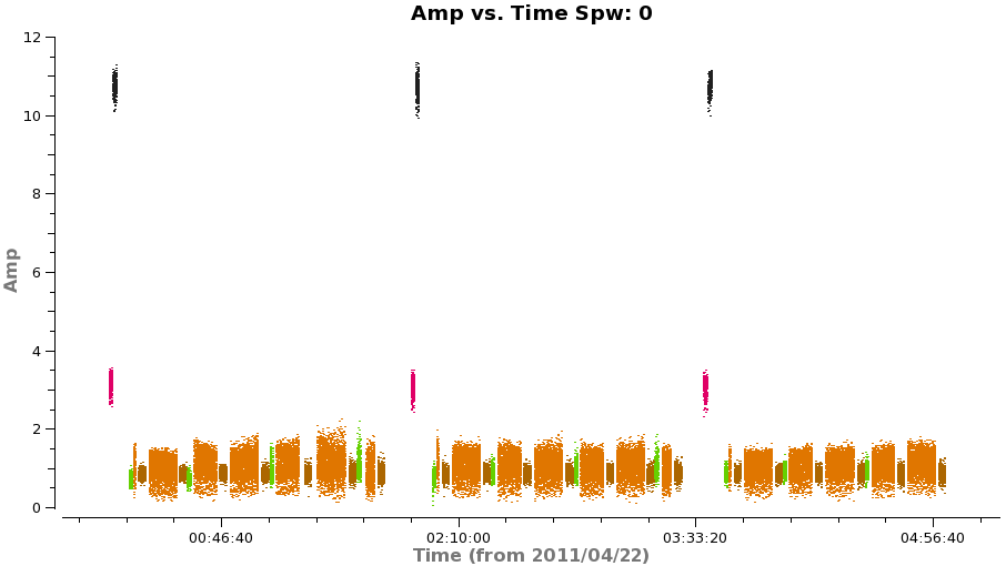
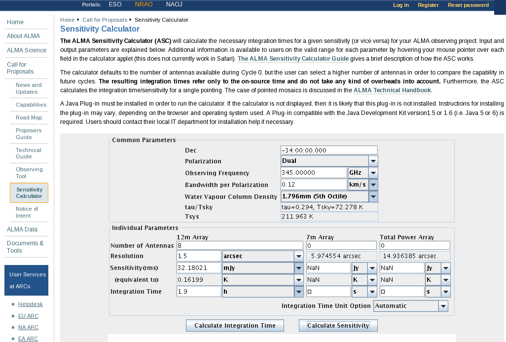
To estimate what the expected noise levels are, we first need to know how much time we had on source. Looking at a plot of amplitude vs time for the concatenated but pre-split data (see below) there are 9x8min scans + 6x6min scans + 3x1min + 2x2min scans for about 1.9 hours on source. There are 2 polarizations and about 1.75 GHz of total continuum bandwidth taking into account flagging.
Using this information and https://almascience.nrao.edu/proposing/sensitivity-calculator, we find that the expected rms noise for the continuum is about 0.3 mJy/beam.
For the spectral line data, which we will image below, with 0.12 km/s channels (needs to be entered in the field bandwidth per polarization), the expected rms noise for the spectral lines is about 32 mJy/beam.
Image and Self-Calibrate the Continuum
Create Initial Clean Image
First we will make an initial image using clean, this task will both deconvolve and clean.
If you are unfamiliar with the basic concepts of deconvolution and clean,
pause here and review for example
http://www.aoc.nrao.edu/events/synthesis/2010/lectures/wilner_synthesis10.pdf
In clean, we use mode='mfs' to do multifrequency synthesis, in other words grid each uv-channel independently. Since the uv-spacing is a function of frequency, this will actually achieve greater uv-coverage than if all the channels and spws had been averaged in advance. The imsize=100 and cellsize=['0.3arcsec'] were chosen to be appropriate for the Band and antenna configuration. At ALMA Band 7, the Full Width Half Power primary beam is about 20", so we want to make our image at least this big. We've made it a bit larger out to about the 25% power point. For the configuration used to take these data, the resolution is expected to be about 1.5" and it is a good idea to oversample the beam by setting the cell size to be a factor of 4 or 5 smaller than the beam (we have used 5 here).
For doing self-calibration it is essential that only "real" signal be included in the image model, thus it is important to make a clean mask, and clean the first iteration rather conservatively (shallowly) so that you are sure that you do not have clean components in your model that do not represent real source emission. In the example below we set interactive=True so you can interactively make the clean mask and stop clean when the signal from the source starts to approach the surrounding "noise" areas in the residual map.
NOTE: Real emission will not go away if you do not put a clean box on it. Conversely if you put a clean box on something that is NOT real and clean deeply you can amplify that feature. Thus, its best to be conservative and build up your clean box as you go, you can generally see fainter "real" features in the residuals.
NOTE: If you start an interactive clean, and then do not make a mask, clean will stop when you tell it to go on because it has nothing to clean. There is no default mask.
<figure id="Viewer_clean1.png">
</figure>
# In CASA
os.system('rm -rf TWHydra_contall.*')
clean(vis='TWHydra_cont.ms',imagename='TWHydra_contall',
      mode='mfs', imagermode='csclean',
      imsize=100,cell=['0.3arcsec'],spw='',
      weighting='briggs',robust=0.5,
      mask='',usescratch=False,
      interactive=True,threshold='1mJy',niter=10000)
NOTE:clean will generate several files automatically with the imagename prepended:
- <imagename>.image # the final restored image
- <imagename>.flux # the effective primary beam response (e.g. for pbcor)
- <imagename>.flux.pbcoverage # the primary beam coverage (ftmachine=’mosaic’ only)
- <imagename>.model # the model image
- <imagename>.residual # the residual image
- <imagename>.psf # the synthesized (dirty) beam
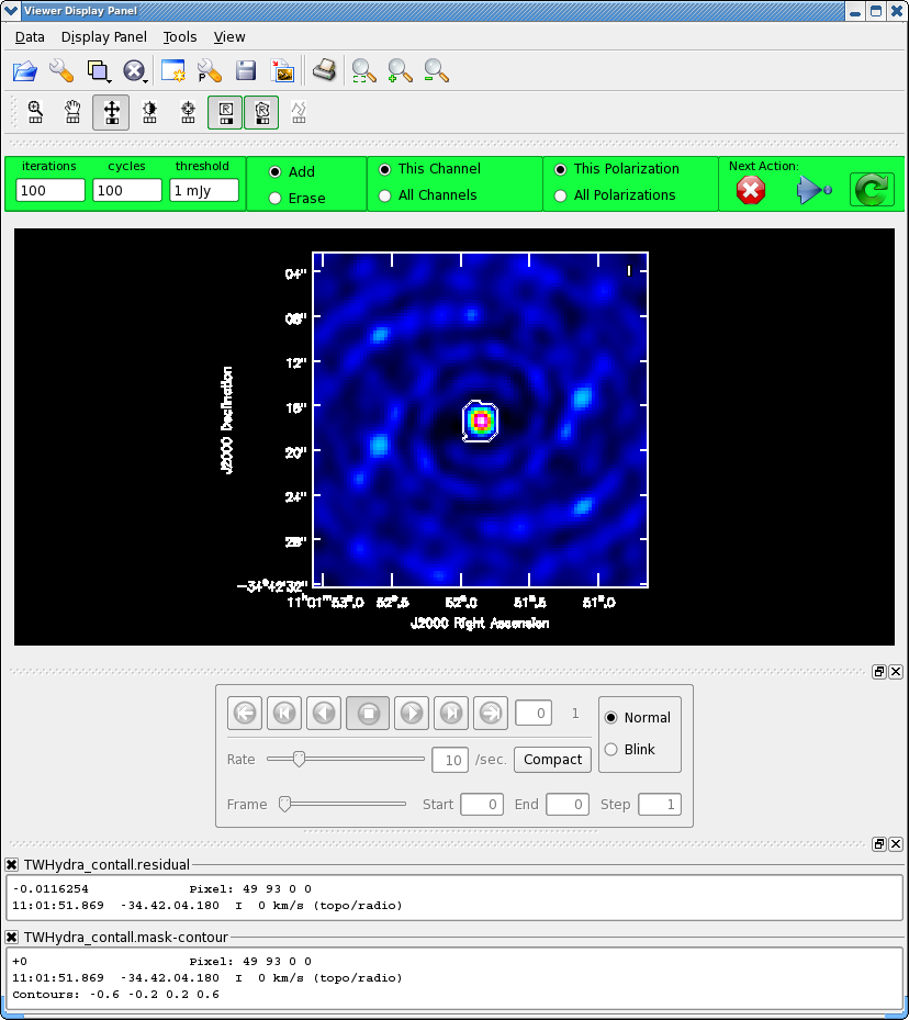
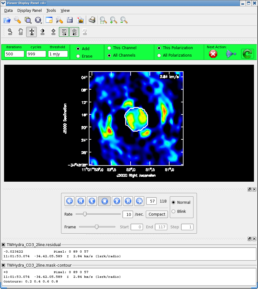
Once the Clean Viewer opens, click on the polygon tool with your left mouse button, and draw a polygon around the continuum emission with the left mouse button. Double click inside the region with the left mouse button when you are happy with it. It will turn from green to white when the clean mask is accepted. To continue with clean use the "Next action" buttons in the green area on the Viewer Display GUI.
The red X will stop clean where you are, the blue arrow will stop
the interactive part of clean, but continue to clean non-interactively
until reaching the number of iterations requested (niter) or the flux
density threshold (whichever comes first), and the green circle arrow
will clean until it reaches the "iterations" parameter on the left side
of the green area.
You should chose the green circle arrow. It will clean 100 iterations (number under iteration in the green area on the Viewer GUI) and then show the residual image again. The middle mouse button is automatically assigned to the "plus" icon, which adjusts the colorscale. If you cannot easily access multiple mouse buttons, you can always assign your one mouse button the icon you want by clicking on it. Adjust the color scale so you can see the structure in the noise better. Also, note that the logger is telling you the amount of clean flux recovered so far, the min/max residuals, and the synthesized beam:
Model 0: max, min residuals = 0.0203454, 0.00267232 clean flux 1.30124
Threshhold not reached yet.
Beam used in restoration: 1.6962 by 1.54549 (arcsec) at pa 28.9043 (deg)
Already with only 100 iterations, the residuals outside the clean mask are larger than that inside. So we will stop here by hitting the Red X symbol.
1st Round of Continuum Data Phase Self-calibration
Next we can use the clean model to self-calibrate the uv-data. The process of self-calibration tries to adjust the data to better match the model you give it. That is why it is important to make the model as good as you can. clean places a uv-model of the resulting image in the file TWHydra_cont.model. This model can then be used to self-calibrate the data using gaincal. We use gaintype='T' to tell it to average the polarizations before deriving solutions (which gains us a sqrt(2) in sensitivity). A critical parameter to play with is solint; we use solint=30s. From listobs the integration time of these data is about 10 seconds, so using solint=30s then gains us a sqrt(3) in sensitivity. It is often best to start with a larger solint and then work your way down to the integration time if the S/N of the data permits. For the same reasons as described in the TWHydraBand7_Calibration_4.5 tutorial we want to fix up the phases before tackling amplitude by setting calmode='p'.
# In CASA
gaincal(vis='TWHydra_cont.ms',caltable='self_1.pcal',
        solint='30s',combine='',gaintype='T',
        refant='DV06',spw='',minblperant=4,
        calmode='p',minsnr=2)
<figure id="Self_1_phase.png">
</figure>
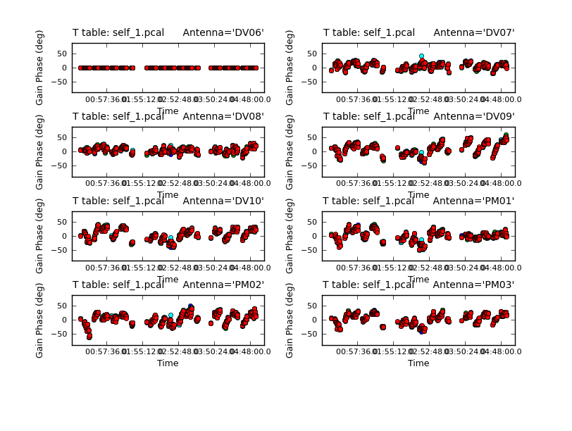
Because combine=' ', we are getting independent solutions for each spw. If you are desperate for S/N, you can try combining them with combine='spw'. We have plenty of S/N in these data so we keep them separate. Look at the solutions.
# In CASA
plotcal(caltable='self_1.pcal',xaxis='time',yaxis='phase',
        spw='',field='',antenna='1~8',iteration='antenna',
        subplot=421,plotrange=[0,0,-80,80],figfile='self_1_phase.png')
The magnitude of corrections gives you a sense of how accurate the phase transfer from the calibrators was. You are checking to see that the phases are being well tracked by the solutions, i.e. smoothly varying functions of time within a given scan. Also the solutions for each spw are lying basically on top of each other which indicates that the spw to spw phase offsets are well calibrated already. Overall, these solutions look quite good. If they didn't you could try increasing the solint and/or combining the spw into a single solution.
After checking that you are happy with the solutions, apply them with applycal
# In CASA
applycal(vis='TWHydra_cont.ms',field='',gaintable=['self_1.pcal'],calwt=False)
<figure id="Viewer_pcal1.png">
</figure>
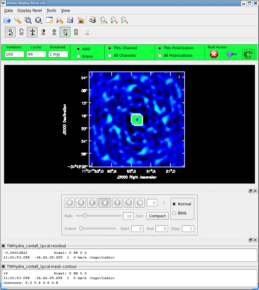
Next clean the source again, to save time we can start with the clean mask from the last iteration. If you make interactive adjustments to the clean mask, they will be written to the new mask TWHydra_contall_1pcal.mask, and not the old one.
# In CASA
os.system('rm -rf TWHydra_contall_1pcal.*')
clean(vis='TWHydra_cont.ms',imagename='TWHydra_contall_1pcal',
      mode='mfs',imagermode='csclean',
      imsize=100,cell=['0.3arcsec'],spw='',
      weighting='briggs',robust=0.5,
      mask='TWHydra_contall.mask',usescratch=False,
      interactive=True,threshold='1mJy',niter=10000)
Now after the first 100 iterations you see that the residuals inside the clean mask are higher than those outside. This is because flux that had been spread out in the map due to poorly correlated phases has been placed where it belongs on the source, thereby increasing its flux. You may also notice that your original clean mask is a little too small. If so, you can make it a bit larger, just by drawing a new polygon around the area you want to include. When you double click, it will incorporate the new mask into the current mask (if your box goes awry you can use the erase toggle [radio button] to erase and redo the mask). The new mask area need not overlap the original mask (though for this source it probably will). You might also want to use the magnifying glass to zoom in. Again, you assign mouse buttons by clicking on the icon you want. Clean another 100 iterations (for a total of 200) and stop by clicking the red X.
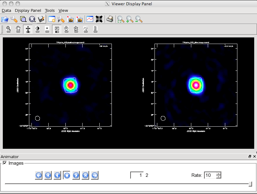
Now open initial and 1st self-cal images to compare them using imview. This is an alternative version of the viewer that is somewhat scriptable.
# In CASA
imview(raster=[{'file':'TWHydra_contall.image','range':[-0.01,0.05]},
       {'file':'TWHydra_contall_1pcal.image','range':[-0.01,0.05]}])
Once the Viewer Display panel opens, click on the box next in the "Images" panel and then use the tapedeck buttons in the panel to alternate between the two images. Because the range was explicitly set, they are on the same color scale. It is obvious that the self-calibrated image is better. To quantify, 1st toggle back to "normal" and then draw a region that excludes the central source with the polygon tool and then double click inside (if you stay in the "Images" view, only the statistics for the last image opened will appear on the terminal instead of both). The basic statistics of the polygon region will print to the terminal:
TWHydra_contall.image
        Stokes       Velocity          Frame        Doppler      Frequency
             I          0km/s           TOPO          RADIO    3.50845e+11
BrightnessUnit       BeamArea           Npts            Sum           Flux
       Jy/beam        33.0039           2357  -9.434800e-01  -2.858690e-02
          Mean            Rms        Std dev        Minimum        Maximum
 -4.002885e-04   7.906752e-03   7.898289e-03  -2.541723e-02   2.172779e-02

TWHydra_contall_1pcal.image
        Stokes       Velocity          Frame        Doppler      Frequency
             I          0km/s           TOPO          RADIO    3.50845e+11
BrightnessUnit       BeamArea           Npts            Sum           Flux
       Jy/beam        33.0039           2357   6.326584e-01   1.916918e-02
          Mean            Rms        Std dev        Minimum        Maximum
  2.684168e-04   3.655786e-03   3.646692e-03  -1.215155e-02   1.109403e-02
The self-calibrated image has more than a factor of 2 lower rms noise!
2nd Round of Continuum Data Phase Self-calibration
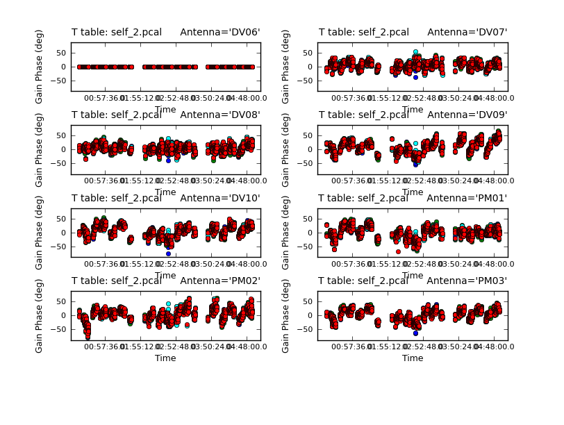
Now that we have a better model, we solve for solutions again. This time we will try making the solint smaller -- the integration time is about 10 seconds, so we set solint='int' to have it use the integration time.
<figure id="Self_2_phase.png">
</figure>
# In CASA
gaincal(vis='TWHydra_cont.ms',caltable='self_2.pcal',
        solint='int',combine='',gaintype='T',
        refant='DV06',spw='',minblperant=4,
        calmode='p',minsnr=2)
Now plot the new solutions.
# In CASA
plotcal(caltable='self_2.pcal',xaxis='time',yaxis='phase',
        spw='',field='',antenna='1~8',iteration='antenna',
        subplot=421,plotrange=[0,0,-80,80],figfile='self_2_phase.png')
The phases on this shorter solint still seem to be tracking well so we will apply it and make a new image and check to see if there is improvement.
# In CASA
applycal(vis='TWHydra_cont.ms',field='',gaintable=['self_2.pcal'],calwt=False)
<figure id="Viewer_pcal2.png">
</figure>
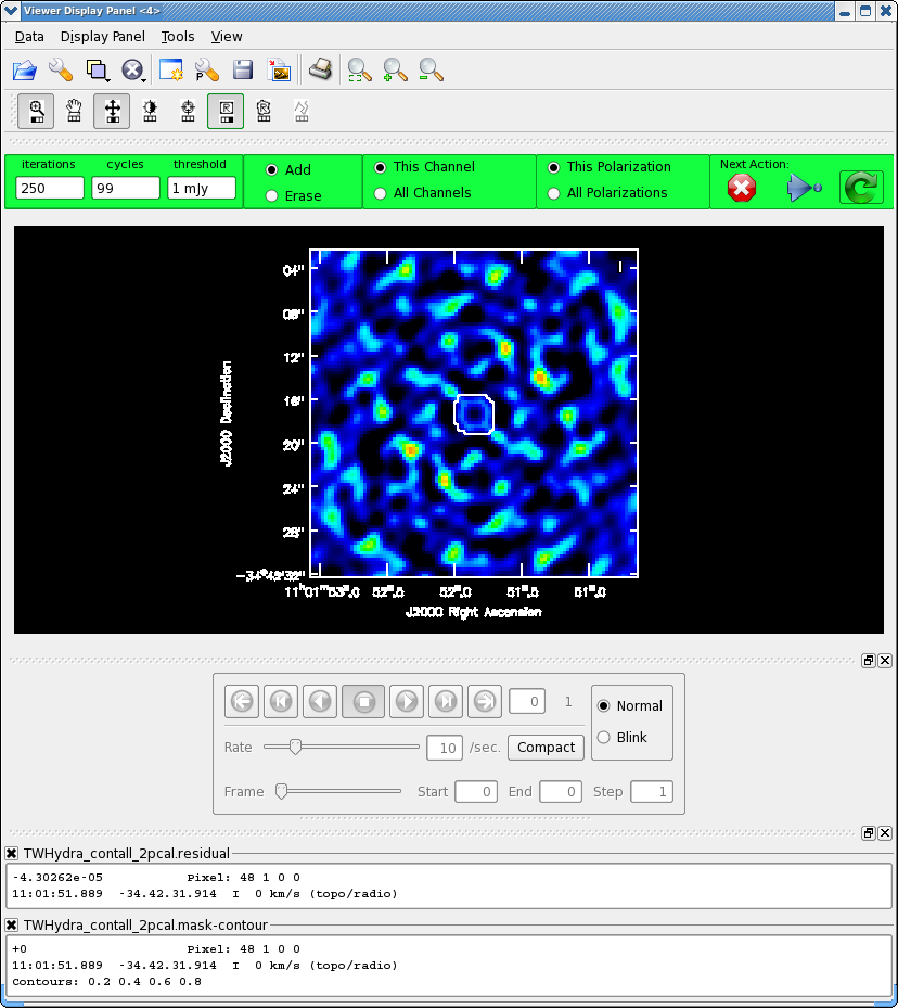
Now clean again, updating mask with the most recent mask file.
# In CASA
os.system('rm -rf TWHydra_contall_2pcal.*')
clean(vis='TWHydra_cont.ms',imagename='TWHydra_contall_2pcal',
      mode='mfs',imagermode='csclean',
      imsize=100,cell=['0.3arcsec'],spw='',
      weighting='briggs',robust=0.5,usescratch=False,
      mask='TWHydra_contall_1pcal.mask',
      interactive=True,threshold='1mJy',niter=10000)
After 200 iterations
Model 0: max, min residuals = 0.00489776, -0.00464541 clean flux 1.44461
It looks like it could use just a little more cleaning, so set iterations=50 in the GUI.
Clean used 50 iterations to approach a threshhold of 0.0015067
0.0107122 Jy <- cleaned in this cycle for  model 0 (Total flux : 1.45532Jy)
Final maximum residual = 0.00326382
Model 0: max, min residuals = 0.00326382, -0.00321361 clean flux 1.45532
The small amount of flux cleaned this cycle indicates that clean is converging and it's about time to stop. Also the residuals inside the clean mask are now smaller than the residuals outside (i.e. the noise) also indicating it's time to stop by hitting the red X on the GUI.
Now repeat the display, blinking, and image statistics steps described above for the 1st and 2nd phase-only self-cal iterations.
# In CASA
imview(raster=[{'file':'TWHydra_contall_1pcal.image','range':[-0.01,0.05]},
       {'file':'TWHydra_contall_2pcal.image','range':[-0.01,0.05]}])
The difference is small:
        Stokes       Velocity          Frame        Doppler      Frequency
             I          0km/s           TOPO          RADIO    3.50845e+11
BrightnessUnit       BeamArea           Npts            Sum           Flux
       Jy/beam        33.0039           2466   4.611597e-02   1.397287e-03
          Mean            Rms        Std dev        Minimum        Maximum
  1.870072e-05   3.831524e-03   3.832255e-03  -1.414417e-02   1.109403e-02

TWHydra_contall_2pcal.image
        Stokes       Velocity          Frame        Doppler      Frequency
             I          0km/s           TOPO          RADIO    3.50845e+11
BrightnessUnit       BeamArea           Npts            Sum           Flux
       Jy/beam        33.0039           2466   1.159416e-01   3.512963e-03
          Mean            Rms        Std dev        Minimum        Maximum
  4.701606e-05   3.811716e-03   3.812199e-03  -1.383034e-02   1.078456e-02
This small improvement suggests that we have gone as far as we can with phase self-cal.
Continuum Data Amplitude Self-Calibration
Now we will apply the best phase solution table on-the-fly while solving for the amplitude self-cal solutions. Since amplitude changes more slowly and is less constrained than phase, we use a longer solint='inf', as long as combine=' ' this means to do one solution per scan.
# In CASA
gaincal(vis='TWHydra_cont.ms',caltable='self_ap.cal',
        solint='inf',combine='',gaintype='T',
        refant='DV06',spw='',minblperant=4,
        gaintable=['self_2.pcal'],
        calmode='ap',minsnr=2)
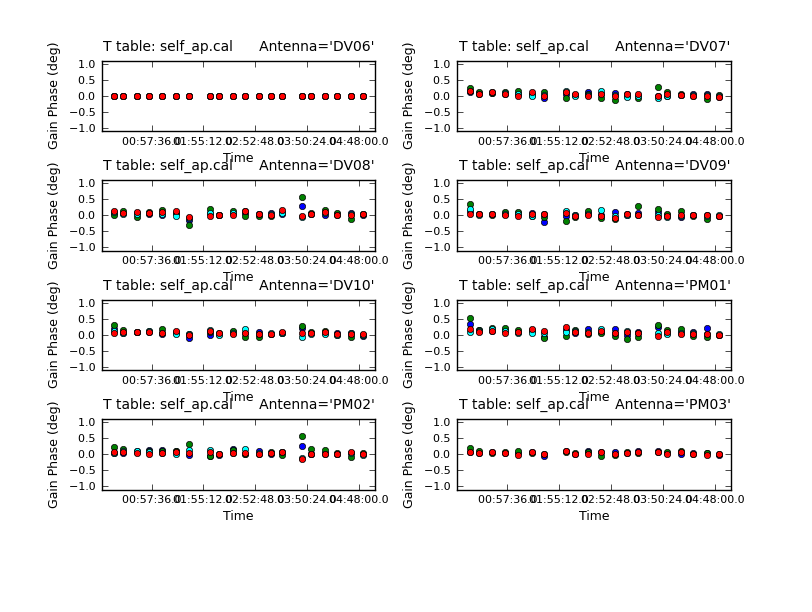
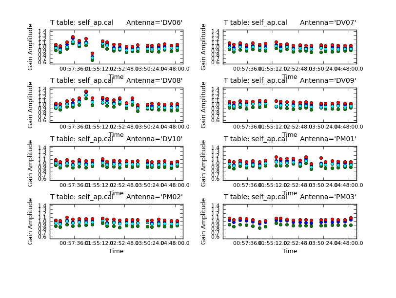
It's useful to look at the residual phase in the amplitude calibration table, i.e. since we applied our best phase-only solution while solving for this new amplitude and phase (calmode='ap') solution, the phase should already be corrected.
<figure id="Self_ap_phase.png">
</figure> <figure id="Self_ap_amp.png">
</figure>
# In CASA
plotcal(caltable='self_ap.cal',xaxis='time',yaxis='phase',
        spw='',field='',antenna='1~8',iteration='antenna',
        subplot=421,plotrange=[0,0,-1,1],figfile='self_ap_phase.png')
The residuals are very small as expected. (If you see large residuals here, it means that the phase-only solution is suspect, and you were mostly just moving noise around.) Now look at the amplitude solutions.
# In CASA
plotcal(caltable='self_ap.cal',xaxis='time',yaxis='amp',
        spw='',field='',antenna='1~8',iteration='antenna',
        subplot=421,plotrange=[0,0,0.6,1.4],figfile='self_ap_amp.png')
For the most part these look very good except one rather large deviation on DV06. Apply both the final phase and the amplitude calibration tables.
# In CASA
applycal(vis='TWHydra_cont.ms',field='',gaintable=['self_2.pcal','self_ap.cal'],calwt=F)
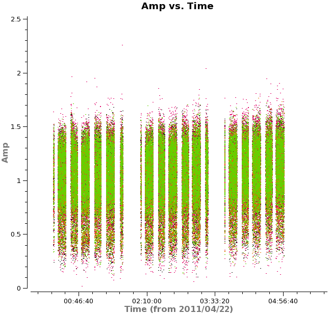
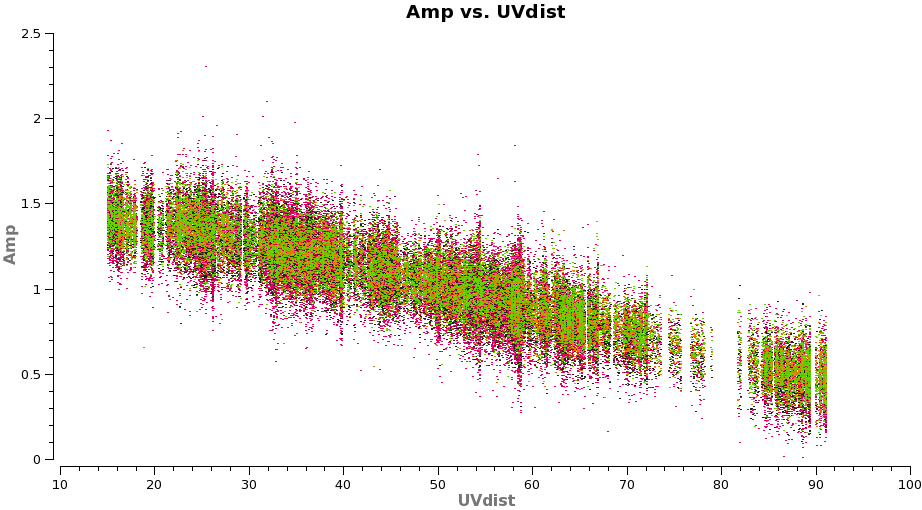
Plot the corrected data as a function of both time and uv-distance. It is always a good idea to check these after an amplitude self-calbration to be sure that it worked properly. Occasionally, a few spurious bits of data will get blown up by the amplitude self-cal if it is not well-constrained.
<figure id="Selfcal_time.png">
</figure> <figure id="Selfcal_uvdist.png">
</figure>
# In CASA
plotms(vis='TWHydra_cont.ms',xaxis='time',yaxis='amp',
       avgchannel='38',ydatacolumn='corrected',coloraxis='spw',
       plotfile='selfcal_time.png')
The time where we saw a large amplitude correction on DV06 looks consistent here so the large correction we saw in the solutions corrected a real issue.
# In CASA
plotms(vis='TWHydra_cont.ms',xaxis='uvdist',yaxis='amp',
       avgchannel='38',ydatacolumn='corrected',coloraxis='spw',
       plotfile='selfcal_uvdist.png')
You will see that this plot looks much better than before.
<figure id="Viewer_apcal.png">
</figure>
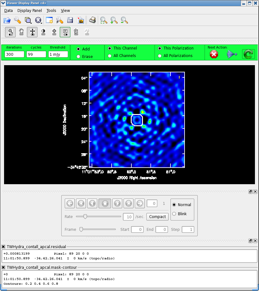
Now make the final continuum image.
# In CASA
os.system('rm -rf TWHydra_contall_apcal.*')
clean(vis='TWHydra_cont.ms',imagename='TWHydra_contall_apcal',
      mode='mfs',imagermode='csclean',
      imsize=100,cell=['0.3arcsec'],spw='',
      weighting='briggs',robust=0.5,usescratch=False,
      mask='TWHydra_contall_2pcal.mask',
      interactive=True,threshold='1mJy',niter=10000)
We know we need to clean with at least 250 iterations (i.e. 100+100+50=250), so set iterations to 300 in the gui and hit the round green arrow. After this notice how much better the residual looks. Clean another 100 iterations. The "circular pattern", and 4 bright spots at each corner you see now in the residual is likely due to non-closing amplitude errors that cannot be removed with an antenna based self-calibration, so this is as good as it gets with pure self-cal. Hit the Red X to stop clean.
Clean used 100 iterations to approach a threshhold of 0.00105507
0.0061808 Jy <- cleaned in this cycle for  model 0
Final maximum residual = 0.00242926
Model 0: max, min residuals = 0.00238278, -0.00242926 clean flux 1.48201
Now repeat the display, blinking, and image statistics described above for the 2nd phase only and the new amplitude & phase self-cal'ed images.
# In CASA
imview(raster=[{'file':'TWHydra_contall_2pcal.image','range':[-0.01,0.05]},
       {'file':'TWHydra_contall_apcal.image','range':[-0.01,0.05]}])
The amplitude and phase self cal'ed image is notably better than phase-only. Quantitatively:
TWHydra_contall_2pcal.image
        Stokes       Velocity          Frame        Doppler      Frequency
             I          0km/s           TOPO          RADIO    3.50845e+11
BrightnessUnit       BeamArea           Npts            Sum           Flux
       Jy/beam        33.0039           3542   2.053068e-01   6.220676e-03
          Mean            Rms        Std dev        Minimum        Maximum
  5.796351e-05   3.955967e-03   3.956101e-03  -1.383034e-02   1.078456e-02

TWHydra_contall_apcal.image
        Stokes       Velocity          Frame        Doppler      Frequency
             I          0km/s           TOPO          RADIO    3.50845e+11
BrightnessUnit       BeamArea           Npts            Sum           Flux
       Jy/beam        33.0039           3542   6.044652e-04   1.831495e-05
          Mean            Rms        Std dev        Minimum        Maximum
  1.706565e-07   1.270183e-03   1.270362e-03  -4.980673e-03   4.137159e-03
and indeed, we've gained another factor of 3 in sensitivity.
Overall with this self-calibration we've improved the noise by a factor of 6.7! With a peak flux density of 0.98 Jy, the S/N increased from 115 initially to 770 after. So, well worth the trouble.
It is notable that we are still a factor of more than 4 from the apriori noise estimate of 0.3 mJy/beam. This is likely due to residual sources of non-closing (not antenna based) errors in the data like baseline errors and baseline-dependent bandpass errors. Additionally, polarization errors (which we did not calibrate at all) can contribute, as well as imperfect uv-coverage with only 8 antennas. A dynamic range of 770 is actually quite good in the submillimeter.
Apply self-calibration to Full Dataset and Split Line Data
Now apply the self-calibration derived from the continuum emission to the full unchannel-averaged data.
# In CASA
applycal(vis='TWHydra_corrected.ms',gaintable=['self_2.pcal','self_ap.cal'],calwt=False)
Split off the CO(3-2) spectral line data in spw=2 and the HCO+(4-3) data in spw=0 for further processing.
# In CASA
os.system('rm -rf TWHydra_CO3_2.ms*')
split(vis='TWHydra_corrected.ms',outputvis='TWHydra_CO3_2.ms',datacolumn='corrected',spw='2')
# In CASA
os.system('rm -rf TWHydra_HCOplus.ms*')
split(vis='TWHydra_corrected.ms',outputvis='TWHydra_HCOplus.ms',datacolumn='corrected',spw='0')
Continuum Subtraction
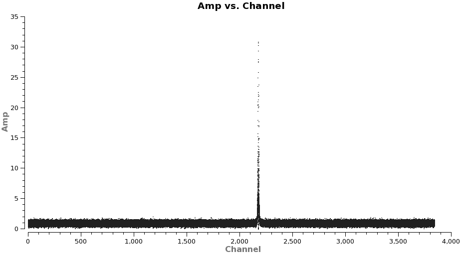
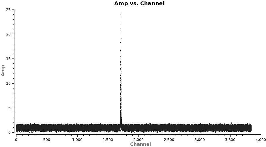
Next we need to subtract the continuum emission from the spectral line data. It is best to do this in the uv-plane. The first step is to make a channel plot of the spectral data to get the line-free channel ranges for both spectral lines. Since the line emission is simple (one spectral line per spw) and there are more than enough line-free channels we do not need to be very precise just stay well away from the line and whenever possible it is best to chose line-free channel ranges on either side of the line for the best possible baseline subtraction.
<figure id="CO3_2_channel.png">
</figure> <figure id="HCOp4_3_channel.png">
</figure>
Note: after the split above, the original spw ids will be relabeled as 0 in each file because there is only one spectral window in each file.
# In CASA
plotms(vis='TWHydra_CO3_2.ms',spw='0',xaxis='channel',yaxis='amp',
      avgtime='1e8',avgscan=True,coloraxis='spw',plotfile='CO3_2_channel.png')
It is a good idea to stay a little away from the very edges of the baseband which can be noisy. The channel ranges 20~2000 and 2400~3800 look like good choices for CO(3-2).
# In CASA
plotms(vis='TWHydra_HCOplus.ms',spw='0',xaxis='channel',yaxis='amp',
      avgtime='1e8',avgscan=True,coloraxis='spw',plotfile='HCOp4_3_channel.png')
The channel ranges 20~1500 and 1900~3800 look like good choices for HCO+(4-3).
Next use the identified line-free channel ranges and uvcontsub to subtract the continuum model from the line emission.
# In CASA
uvcontsub(vis='TWHydra_CO3_2.ms',fitorder=1,fitspw='0:20~2000,0:2400~3800')
# In CASA
uvcontsub(vis='TWHydra_HCOplus.ms',fitorder=1,fitspw='0:20~1500,0:1900~3800')
Note: If you do not have line-free channels on both sides of the line emission, it is safer to use fitorder=0, or the fit may diverge.
Spectral Line Imaging
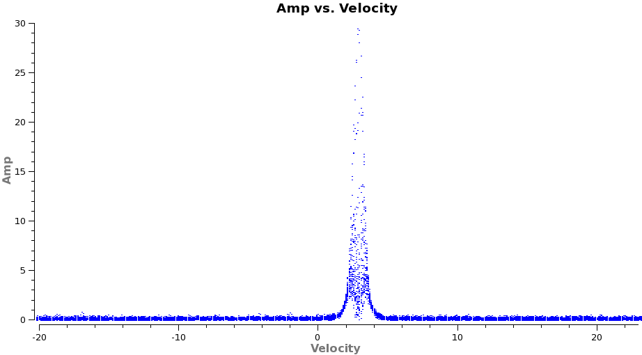
Now we are ready to make cubes of the line emission. The imaging parameters are similar to the continuum except for those dealing with the spectral setup: mode, start, width, nchan, restfreq, and outframe parameters. When making spectral images you have three choices for the mode parameter: channel, velocity, and frequency. Data are taken using constant frequency channels. For spectral line analysis it's often more useful to have constant velocity channels, and this is also the best way to make images of multiple lines with the exact same channelization for later comparison. For mode='velocity', the desired start and width also need to be given in velocity units for the desired output frame.
It is important to note that ALMA does not do on-line Doppler Tracking and the native frame of the data is TOPO. If you do not specify outframe the output cube will also be in TOPO, which is not very useful for spectral line work. The Doppler Shift is taken out during the regridding to the desired outframe in clean or alternatively it can be done separately by the cvel task which would need to be run before clean.
<figure id="CO3_2_vel.png">
</figure> <figure id="HCOp4_3_vel.png">

</figure>
To see what velocity parameters you want to set in clean it is useful to make a plot in plotms in the desired output frame. To make it easier to see, we set a plotrange since we know the LSRK velocity of TW Hya is about 2.88 km/s. Note these plots take a little longer because of the frame shift.
# In CASA
plotms(vis='TWHydra_CO3_2.ms.contsub',xaxis='velocity',yaxis='amp',
       avgtime='1e8',avgscan=True,transform=True,freqframe='LSRK',
       restfreq='345.79599GHz',plotrange=[-20,23,0,0],plotfile='CO3_2_vel.png')
# In CASA
plotms(vis='TWHydra_HCOplus.ms.contsub',xaxis='velocity',yaxis='amp',
      avgtime='1e8',avgscan=True,transform=True,freqframe='LSRK',
      restfreq='356.7342GHz',plotrange=[-20,23,0,0],plotfile='HCOp4_3_vel.png')
From these plots it looks like imaging the cubes from about -5 to +8 km/s will encompass the line, but still provide several line-free channels on either side so the noise level can be estimated. The channel width is 122 kHz, which at 345.79599 GHz is 0.106 km/s. Recall that the spectral resolution is a factor of two poorer. We will use a velocity channel width of 0.12 km/s for a little oversampling, but the spectral resolution remains 0.2 km/s.
As before, it is very important that you make a clean mask. There are many ways to do this ranging from the complicated to simple. For this example we will make a single clean mask that encompasses the line emission in every channel and apply it to all channels. This is much better than no clean mask, though not quite as good as making an individual mask for each channel. For some sources, one can use the continuum mask to clean the line, however TW Hya is a bit curious in that the continuum emission is not as extended as the line emission (Hughes et al. 2008).
CO(3-2) Imaging
# In CASA
os.system('rm -rf TWHydra_CO3_2line.*')
clean(vis='TWHydra_CO3_2.ms.contsub',imagename='TWHydra_CO3_2line',
      imagermode='csclean',spw='',
      imsize=100,cell=['0.3arcsec'],
      mode='velocity',start='-4km/s',width='0.12km/s',nchan=118,
      restfreq='345.79599GHz',outframe='LSRK',
      weighting='briggs',robust=0.5,
      mask='',usescratch=False,
      interactive=True,threshold='1mJy',niter=100000)
<figure id="Viewer_55.png">
</figure> <figure id="Viewer_500.png">
</figure>
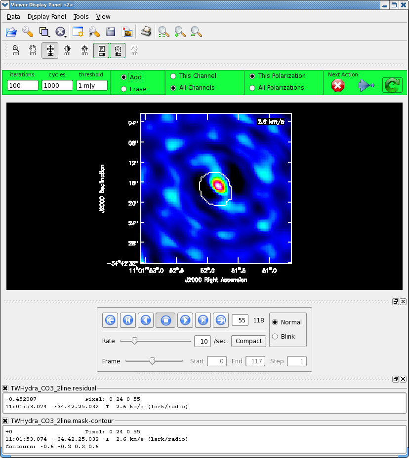
It will take a little while to grid the cube, when the interactive viewer opens, use the tapedeck to cycle through the channels. You should see a progress of line emission in channels 40 to 70 or so.
- Go to channel 57 (about line center)
- Select the polygon tool with the left mouse button
- Select the "All Channels" toggle in the green area
- Draw a polygon around the channel 57 emission, double click inside to activate.
- Now go to channel 60, this is the channel with the most extent to the SE, draw another polygon that encompasses this emission if necessary,double click inside to activate.
- Now go to channel 55, this is the channel with the most extent to the NW, draw another polygon that encompasses this emission if necessary,double click inside to activate.
- Now double check the mask by cycling through channels with real line emission to be sure that your clean box encompasses the emission, but does not extend far beyond it. Again the "erase" toggle can come in handy if things go awry or if you want to just delete a small portion of an existing mask (just draw a polygon around what you want to erase and double click inside), be sure to switch back to "add" before going on.
The figure shows what the final clean box should look like. Now clean using the green circle arrow. You can watch the progress in the logger. When 100 iterations are done, the viewer will show the residual map for each channel. Cycle through the channels and see whether you are still happy with the clean box in each signal channel. The "erase button" can help you fix mistakes. If necessary adjust. It is often useful to adjust the colorscale with the "plus" symbol icon. Keep going until the residual emission looks like the surrounding noise. If it seems to be going slowly, increase the iterations to 300 for a round or two. I stopped cleaning (Red x) when the logger showed (about 900 iterations).
12.9846 Jy <- cleaned in this cycle for  model 0
Final maximum residual = 0.157312
Model 0: max, min residuals = 0.157312, -0.0871295 clean flux 279.304
NOTE: The residuals are still a bit high in the strongest emission channels after it is well cleaned in the weaker channels. This is an indication that the sensitivity is "dynamic range" limited. In other words even with more intrinsic sensitivity per integration (i.e. better system temperature), the dynamic range limit would remain the same unless you get more uv-coverage. The fundamental dynamic range limitations of ALMA will be considerably better with 16 antennas in Early Science and MUCH better with the full 50-antenna array.
HCO+(4-3) Imaging
Now image and clean the HCO+(4-3) line using what you learned above.
# In CASA
os.system('rm -rf TWHydra_HCOplusline.*')
clean(vis='TWHydra_HCOplus.ms.contsub',imagename='TWHydra_HCOplusline',
      imagermode='csclean',spw='',
      imsize=100,cell=['0.3arcsec'],
      mode='velocity',start='-4km/s',nchan=118,width='0.12km/s',
      restfreq='356.7342GHz',outframe='LSRK',
      weighting='briggs',robust=0.5,
      mask='',usescratch=False,
      interactive=True,threshold='1mJy',niter=100000)
I stopped cleaning when:
4.79833 Jy <- cleaned in this cycle for  model 0
Final maximum residual = 0.0977348
Model 0: max, min residuals = 0.0977348, -0.060484 clean flux 192.066
Image Analysis
After all that hard work you now have deconvolved images of the 350 GHz continuum, the CO (3-2) line, and the HCO+ (4-3) line. CASA includes tools to help you understand the contents of these images and make basic scientific measurements. These tools are divided between graphical exploration tools, accessible via the CASA viewer, and command line analysis tasks. To access the viewer, simply type viewer() and to see the list of analysis tasks available in CASA type tasklist at the CASA prompt and look under the Analysis sub-heading.
If you want to do this portion of the guide and have downloaded the (.FITS) reference images, you can import them to be CASA images using importfits. If you are re-importing the images, use the commented remove command, here, to delete the previous import first.
# In CASA
# os.system("rm -rf TWHydra_CO3_2line.image")
importfits(fitsimage="TWHydra_CO3_2line.image.fits", imagename="TWHydra_CO3_2line.image")
where fitsimage refers to the file to imported and imagename gives the output filename. If you are proceeding directly from the imaging step, your data are already CASA images and you may proceed without any importing.
You can get the basic properties of any CASA image using the imhead command. For example, type
# In CASA
imhead("TWHydra_CO3_2line.image")
and look at the CASA logger. You will see an image summary like the following
INFO imhead	##########################################
INFO imhead	##### Begin Task: imhead             #####
INFO imhead	imhead(imagename="TWHydra_CO3_2line.image",mode="summary",hdkey="",hdvalue="",
INFO imhead	        hdtype="",hdcomment="",verbose=False)
INFO ImageAnalysis
INFO ImageAnalysis	Image name       : TWHydra_CO3_2line.image
INFO ImageAnalysis	Object name      : TW Hya
INFO ImageAnalysis	Image type       : PagedImage
INFO ImageAnalysis	Image quantity   : Intensity
INFO ImageAnalysis	Pixel mask(s)    : None
INFO ImageAnalysis	Region(s)        : None
INFO ImageAnalysis	Image units      : Jy/beam
INFO ImageAnalysis	Restoring Beam   : 1.68065 arcsec, 1.53193 arcsec, 22.3015 deg
INFO ImageAnalysis
INFO ImageAnalysis	Direction reference : J2000
INFO ImageAnalysis	Spectral  reference : LSRK
INFO ImageAnalysis	Velocity  type      : RADIO
INFO ImageAnalysis	Rest frequency      : 3.45796e+11 Hz
INFO ImageAnalysis	Pointing center     :  11:01:51.844983  -34.42.17.160885
INFO ImageAnalysis	Telescope           : ALMA
INFO ImageAnalysis	Observer            : Unknown
INFO ImageAnalysis	Date observation    : 2011/04/22/00:15:42
INFO ImageAnalysis	Telescope position: [2.22514e+06m, -5.44031e+06m, -2.48103e+06m] (ITRF)
INFO ImageAnalysis
INFO ImageAnalysis	Axis Coord Type      Name             Proj Shape Tile   Coord value at pixel      Coord incr Units
INFO ImageAnalysis	--------------------------------------------------------------------------------------------------
INFO ImageAnalysis	0    0     Direction Right Ascension   SIN   100   25  11:01:51.845    50.00   -3.000000e-01 arcsec
INFO ImageAnalysis	1    0     Direction Declination       SIN   100   25 -34.42.17.161    50.00    3.000000e-01 arcsec
INFO ImageAnalysis	2    2     Spectral  Frequency               118   59   3.45801e+11     0.00 -1.38414152e+05 Hz
INFO ImageAnalysis	                     Velocity                                    -4     0.00    1.200000e-01 km/s
INFO ImageAnalysis	3    1     Stokes    Stokes                    1    1             I
INFO imhead	##### End Task: imhead               #####
INFO imhead	##########################################
This report tells you about the target, shape, and coordinates of the image. It also notes the rest frequency and some details of the observation. imhead may be used more generally to retrieve header keywords as python variables or to manipulate the header of an image. Consult the help for details.
You may want to pay particular attention to the third and fourth axis of the CASA image. These are
usually frequency (velocity) and Stokes (polarization) in some order. An occasional source of confusion
is that this order is not always the same. Often CLEAN will output images with the Stokes axis third,
while IMPORTFITS usually yields images with the frequency axis third. If you encounter problems with
image analysis tasks, you may want to check whether this results from conflicting axis definitions. You
can adjust the order of the axes using the IMTRANS task.
Before proceeding, make sure that you have all three data sets as CASA images: TWHydra_CO3_2line.image, TWHydra_HCOPlusline.image, and TWHydra_contall_apcal.image. If you do not, then import them from the provided reference images. If you are re-importing the FITS images, run the commented remove commands before running importfits.
# In CASA
# os.system("rm -rf TWHydra_CO3_2line.image")
importfits(fitsimage="TWHydra_CO3_2line.image.fits", imagename="TWHydra_CO3_2line.image")
# os.system("rm -rf TWHydra_HCOplusline.image")
importfits(fitsimage="TWHydra_HCOplusline.image.fits", imagename="TWHydra_HCOplusline.image")
# os.system("rm -rf TWHydra_contall_apcal.image")
importfits(fitsimage="TWHydra_contall_apcal.image.fits", imagename="TWHydra_contall_apcal.image")
In the rest of this guide we will construct moment maps showing the integrates, velocity field, and line width of the two lines. We will carry out Gaussian fits to the continuum and line maps. We will also illustrate some of the additional analysis capabilities available in CASA: subcube extraction, retrieval of data into python arrays, cube alignment, smoothing, and overlays of multiple spectral lines.
Moment Maps
The line "images" of CO(3-2) and HCO+(4-3) are, of course, cubes rather than images. Two dimensional moment maps are a standard way to present such data. These are maps showing the result of various moments (or similar calculations) carried out along the frequency axis of the cube. For example, the "moment 0" map is the sum of emission along the frequency axis at each pixel. The first moment is the intensity-weighted velocity (or frequency). The second moment is the intensity-weighted velocity (or frequency) dispersion about the mean. These and a number of other calculations (for example the maximum intensity) can be calculated via the immoments task. Consult the help or the CASA cookbook for more details.
In this section, we will calculate moments for our two spectral line data cubes. To make the highest quality moment maps, we will first identify the planes of the data cube that contain emission, so that we can carry out the sum only over these channels. Doing otherwise adds noise to the moment map without adding signal and so lowers the signal-to-noise ratio of the final image. For the first and second moments we will identify an intensity threshold above which the data are statistically very likely to correspond to real astronomical emission. We will restrict the calculation to consider only data above this threshold, yielding a cleaner calculation (the second moment, in particular, is not at all robust against the inclusion of outlying noise). Finally, we will inspect the resulting moment maps with the viewer and output them to .FITS files.
Estimate the Spectral Extent
First, we want to figure out what planes appear to contain real emission. Open the CO data cube with the CASA viewer via:
# In CASA
viewer("TWHydra_CO3_2line.image")
This will open the CO(3-2) data cube as a raster image. Use the Animator pane to scroll through the cube, noting that the emission is mostly confined to ~40 channels near the center of the cube. There are several ways to make a more rigorous estimate.
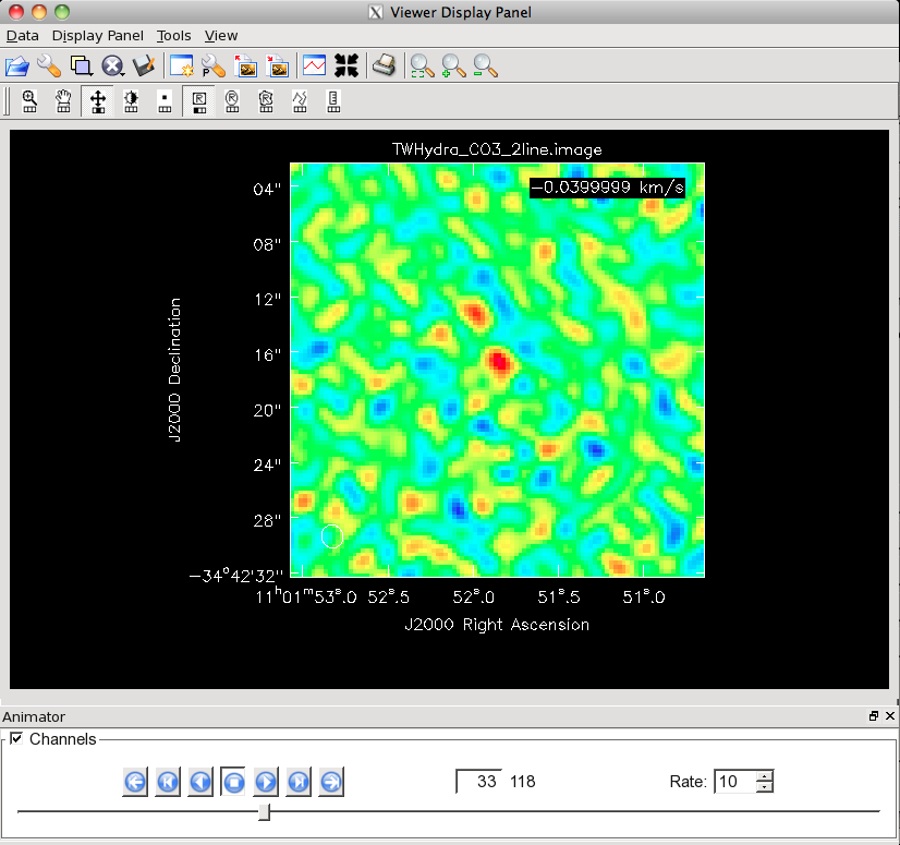
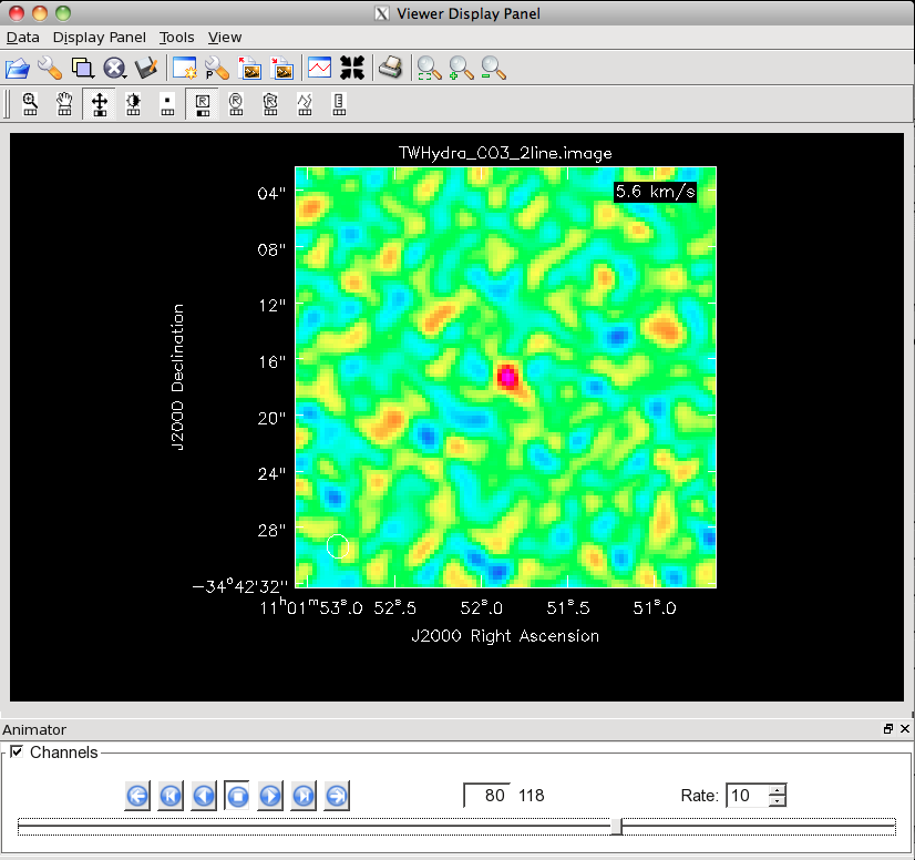
By-Plane Inspection: First, you could increase the stretch of the image to identify by hand the first and last channels with visible emission. To do open the Data Display Options panel in the viewer (the wrench icon) and manually set the data range and/or scaling power cycles to highlight faint emission (note that you can also do this using the mouse and the color stretch - sun - icon). I left the scaling power cycles at 0 and set the data range to [-0.15, 0.15]. Then scroll through the cube and note the first and last channels with obvious emission. If I do this, I find emission from about plane 30 through plane 86.
-
The Data Display Panel used to set the color stretch, here from [-0.15, 0.15] with a linear (0) stretch. Setting the stretch to a negative value will highlight lower emission (a more logarithmic stretch). We got to this panel by clicking the wrench icon. You can also get from the dropdown menus (Data->Adjust).
-
Channel 33 of the CO(3-2) cube on this stretch. This is about the first channel to show clear emission.
-
Channel 80 of the CO(3-2) cube on this stretch. This is about the last channel to show clear emission.
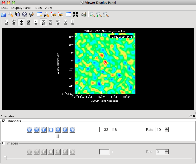
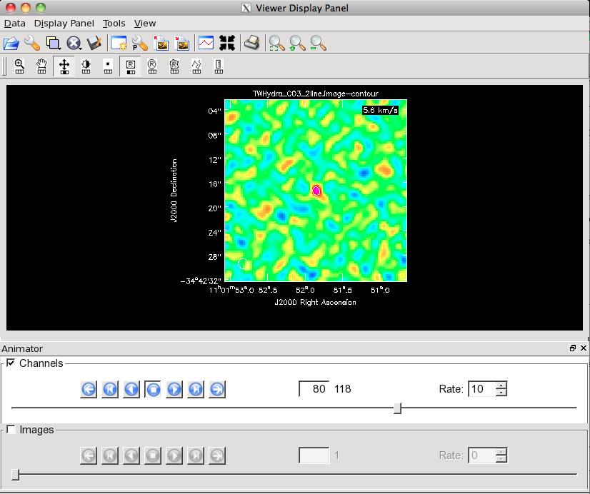
To make this more rigorous, you can work out a noise estimate before hand (we'll find it to be about 0.025 Jy/beam) and overplot a contour to indicate significant emission. You can do this by hand by using the Data Manager (folder icon) to open TWHydra_CO3_2line.image as a "contour map" and then using the Data Display Options to manipulate the contour levels. To show a 3-sigma contour with sigma=0.025 Jy/beam set the Relative Contour Levels to [3], the Base Contour Level to 0, and the Unit Contour Level to 0.025. You can display a 5-sigma contour or change the RMS analogously. Scrolling through the cube, I see 3-sigma emission from channels 33 through 80.
-
The Data Display Panel now being used to set the contour levels. We set the contour unit to 0.025 and ask for a single contour at 3 times this value. Notice that we clicked the tab along the top of the window to select the contour map.
-
Channel 33 of the CO(3-2) cube on this stretch with a 3-sigma contour overlaid.
-
Channel 80 of the CO(3-2) cube on this stretch with a 3-sigma contour overlaid.
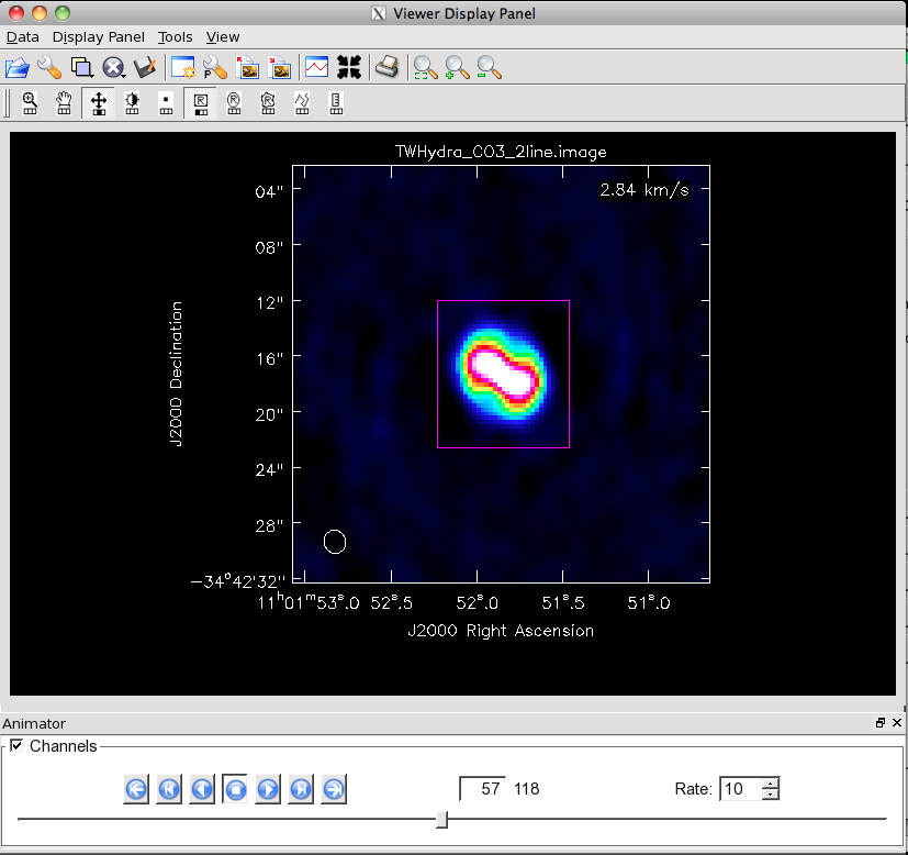
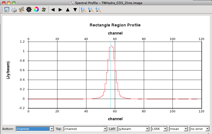
Look at a Spectrum: You can also look at a spectrum of the source. To do this, scroll to a channel with a lot of emission (I went to 57) and then use the mouse to drag out a rectangle. To do this, left click on the rectangle box in the mouse toolbar (this assigns the left mouse button to define rectangle regions). Then drag out a box around the emission using the same button. Now click the spectrum in the toolbar to open the spectral profile tool. You will see the average profile for the selected region. You can set the bottom axis to show channels. You can zoom in within the spectral profile by dragging out a rectangle. When I do this, I find significant emission from channels 40-80.
-
Defining a rectangular region around the main emission from TW Hydra. First we clicked the rectangle button on the mouse toolbar, then we held that button and dragged out the purple rectangle. After defining the rectangle, you can drag it around or delete it with <ESC>.
-
The spectrum of this rectangular region viewed in the spectral profile browser. Note that the bottom axis has been set to show channels. To get this spectrum, we defined the rectangular region and then clicked the spectrum button on the toolbar.
-
A zoom in on the spectrum. The line extends from channels ~40-80.
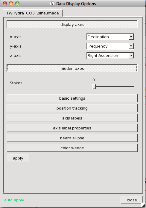
Look at a Declination-Frequency Projection (or an R.A.-Frequency Projection): This is probably the least reliable way to do this, but illustrates a neat capability of the viewer. Open the Data Display Options (click the wrench icon) and open the "display axes" and "hidden axes" tabs. Use the dropdown menus to change the display so that the x-axis shows Declination, the y-axis shows Frequency, and the z-axis shows "Right Ascension." Now you are scrolling through planes of intensity as a function of Declination and Frequency. Use the animator to move to R.A. plane ~ 50 (the center of the source) and pull the stretch up (in the wrench tool; I used [-0.15,0.15] again). Mouse over the image and look at the "Position Tracking" pane in the bottom of the image, noting the pixel extent of emission in the frequency axis of this plane. I see traces of emission from channel ~30-90.
-
The Data Display Panel, here used to set which axes are displayed. We have adjusted the y-axis to show frequency and the x-axis to show Declination. The z-axis is now Right Ascension, so that we will scroll through planes of Right Ascension.
-
The Data Display Panel, here we are setting coordinates to show "pixels" rather than world coordinates.
-
A Frequency-Declination plane of the cube near the central R.A. pixel (50). The rough extent of emission may be simply read off the y-coordinate. As above, we could overplot a 3-sigma contour to add more rigor.
You can repeat this exercise for the HCO+ (4-3) emission. Using the Spectral Profile Browser, I find that the line extends from about channel 40 through channel 75.
Make Moment 0 Maps
With an estimate of the spectral extent of emission, we are now ready to make moment 0 maps of the CO(3-2) and HCO+(4-3) lines. It is possible to do this using the 'Calculate Moments/Spectral Profile tool' in the viewer, but here we do this using the immmoments command,
# In CASA
os.system('rm -rf TWHydra_CO3_2line.image.mom0')
immoments(imagename='TWHydra_CO3_2line.image',moments=[0],
          outfile='TWHydra_CO3_2line.image.mom0',
          chans='30~90')
and
# In CASA
os.system('rm -rf TWHydra_HCOplusline.image.mom0')
immoments(imagename='TWHydra_HCOplusline.image',moments=[0],
          outfile='TWHydra_HCOplusline.image.mom0',
          chans='40~75')
immoments will sum across the channels specified by chans and produce new CASA images with the names specified by outfile. These can be inspected using the CASA viewer just like any other image. Note that unlike higher-order moments, the moment-0 map is robust to the inclusion of noisy signal-free channels (to within reason, you just decrease your signal-to-noise ratio) and indeed may be biased to miss faint emission by imposing a threshold. For that reason, we will eschew the includepix keyword as we make the moment 0 maps.
Let's look at the output using the viewer. We can specify some of the display options in the call to start the viewer by using imview instead of viewer.
# In CASA
imview( raster=[ {'file':'TWHydra_CO3_2line.image.mom0',
                  'range':[0.0,10.],
                  'scaling':-1},
                 {'file':'TWHydra_HCOplusline.image.mom0',
                  'range':[0.0,10.],
                  'scaling':-1}],
         contour={'file':'TWHydra_contall_apcal.image', 'base':0, 'unit':0.0025, 'levels':[3,100]} )
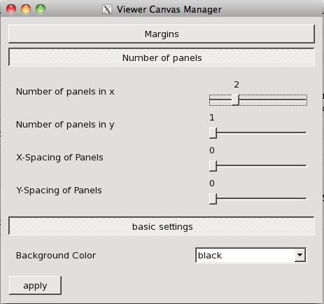
This does several things: It opens the viewer with raster images of the moment 0 maps of CO(3-2) and HCO+(4-3), sets the range of the color stretch from [0, 10] for each image and sets the scaling to be -1, which highlights faint emission compared to the normal (0) stretch. It also opens the continuum image as a contour and defines two contour levels. Once the viewer is open, you can blink between the images by going into the Animator pane, checking the white box next to "Images" to enable animation between images, and then sliding the bar back and forth. See the name of the image being shown change. You can also show two images side by side by going to the Viewer Canvas Manager (wrench+P icon) and opening the "Number of Panels" tab. Set the "Number of panels in x" to 2 and make sure that the Images box is checked in the Animator pane. You will see both images side by side.
-
The Viewer Canvas Manager, accessed via the Wrech+P icon (not to be confused with the plain old wrench). Here we have adjusted the number of x-panels from 1 to 2 so that we show the two moment maps side by side.
-
The moment-0 maps of CO(3-2) and HCO+(4-3) plotted side by side on the same color stretch, both with the continuum contours overlaid. To get the two images side by side, run the imview call above then set the number of panels to 2 and make sure that the Images box in the Animator Pane (here at the bottom of the window) is checked.
-
Data Display Panel after our imview call. Imview allowed us to set the stretch, range, and contour levels from the command line.
Estimate the Noise
We have already made a few offhand comparisons to the RMS noise. This quantity is often critical to know when exploring the data. Because the higher-order moments (especially the dispersion) are not at all robust to the inclusion of noise, we will calculate them only from regions of the cube that have intensity several times the RMS noise value or higher and are thus very likely to contain real astronomical emission. To proceed, we need to estimate the RMS noise for our data.
The easiest way to do this is to calculate the RMS scatter of the data about zero from a part of the data that you suspect to be (mostly) free of astronomical signal. In a data cube the easiest way to do this will often be to identify signal-free planes (channels) of the cube -- we use channel 25 in the example below -- and to simply calculate the RMS in these regions. We can do this straightforwardly using the imstat command in CASA.
# In CASA
imstat('TWHydra_CO3_2line.image',chans='25')
The output will look like this (note that the rms is just one line in the returned array):
{'blc': array([ 0,  0, 25,  0], dtype=int32),
 'blcf': '11:01:53.061, -34.42.32.161, 3.457971e+11Hz, I',
 'flux': array([ 0.04564727]),
 'max': array([ 0.07162448]),
 'maxpos': array([19, 20, 25,  0], dtype=int32),
 'maxposf': '11:01:52.599, -34.42.26.161, 3.457971e+11Hz, I',
 'mean': array([ 0.00014796]),
 'medabsdevmed': array([ 0.01346229]),
 'median': array([-0.00012413]),
 'min': array([-0.08078942]),
 'minpos': array([49, 19, 25,  0], dtype=int32),
 'minposf': '11:01:51.869, -34.42.26.461, 3.457971e+11Hz, I',
 'npts': array([ 10000.]),
 'q1': array([-0.01331472]),
 'q3': array([ 0.01357804]),
 'quartile': array([ 0.02689276]),
 'rms': array([ 0.02048737]),
 'sigma': array([ 0.02048786]),
 'sum': array([ 1.47963354]),
 'sumsq': array([ 4.19732144]),
 'trc': array([99, 99, 25,  0], dtype=int32),
 'trcf': '11:01:50.653, -34.42.02.461, 3.457971e+11Hz, I'}
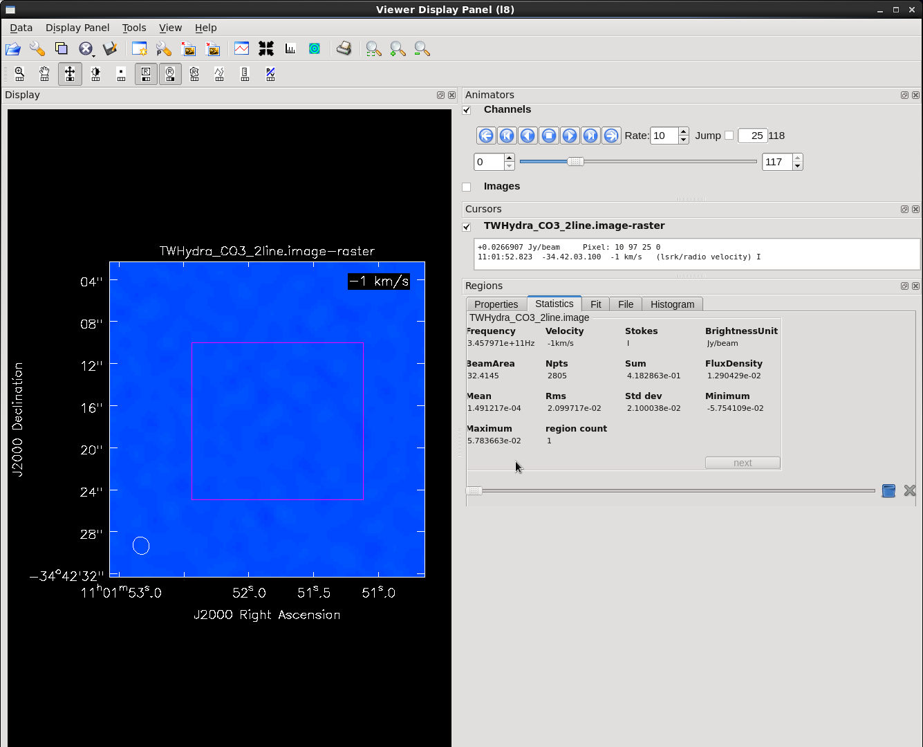
Alternatively, you can get similar statistics on a region of an image or data cube selected manually inside the viewer. Drag out a region, for example a rectangle, using one of the mouse tools; the box that you draw will be purple (the zoom button gives you a green box!) Make sure that "Regions" is checked under the View menu, and then your region's statistics will show up in the viewer itself, as shown in the Figure.
<figure id="Twhydra_region.png">
</figure>
(Suggested values for CO(3-2), HCO+(4-3), and continuum.)
Since errors in calibration must result in errors in the image plane, and these behave like sidelobes of the beam in that they move power away from the peak into the rest of the map in a given channel, we measure the rms in a line-free channel. By avoiding channels where there is real (especially bright) emission, we avoid measuring these errors as a true rms in the image. This is called being dynamic range limited. If, for instance, the calibration is only good to a few percent, then when the ratio of the peak brightness to the rms noise measured in a line free channel is a hundred or more, the rms noise in line-full channels will increase relative to the line-free ones. You can see this in the TWHydra_CO3_2line.image cube.
Note that generally we want to measure the characteristic rms noise in an image before the correction for the response of the instrument
(remember the mention of the .flux image above), which is called the primary beam correction. Before a primary beam correction, the noise
is consistent across the image and reflects the quality of the calibration and imaging, which is generally what we want to know when we
measure the rms. Afterward, it also includes the direction-dependent instrument response, or the falloff in sensitivity as you move away
from the phase center. This correction is necessary to assess how much of your structure has been detected at high signal-to-noise (if the
source is extended well beyond the phase center -- note that TWHydra is not); accurate flux measurements of extended emission can only
be made using the corrected image.
Higher Order Moment Maps for CO(3-2)
For higher order moments it is very important to set a conservative flux threshold. Typically something like 6 sigma, using sigma from peak line channel, works well.
# In CASA
os.system('rm -rf TWHydra_CO3_2line.image.mom')
os.system('rm -rf TWHydra_CO3_2line.image.mom.weighted_coord')
os.system('rm -rf TWHydra_CO3_2line.image.mom.weighted_dispersion_coord')
immoments(imagename='TWHydra_CO3_2line.image',moments=[1,2],
          outfile='TWHydra_CO3_2line.image.mom',
          chans='40~76',includepix=[0.3,100])
Display all three moment maps in the viewer, overlaid with continuum contours.
# In CASA
imview( raster=[ {'file':'TWHydra_CO3_2line.image.mom0'},
                 {'file':'TWHydra_CO3_2line.image.mom.weighted_coord'},
                 {'file':'TWHydra_CO3_2line.image.mom.weighted_dispersion_coord'} ],
        contour={'file':'TWHydra_contall_apcal.image', 'base':0, 'unit':0.0025, 'levels':[3,100]} )
To see all three raster images simultaneously, open the viewer's Panel Display Options (the "P-wrench" icon in the viewer tool bar), click "Number of panels", and change "Number of panels in x" to 3. Then select the "Blink" toggle (radio button) from the Animator panel.
<figure id="TWHya_CO3_2_moments.png">

</figure>
Repeat for HCO+(4-3) which has a bit narrower velocity extent than the CO(3-2), but similar rms noise.
# In CASA
os.system('rm -rf TWHydra_HCOplusline.image.mom0')
immoments(imagename='TWHydra_HCOplusline.image',moments=[0],
          outfile='TWHydra_HCOplusline.image.mom0',
          chans='43~74')
# In CASA
os.system('rm -rf TWHydra_HCOplusline.image.mom')
os.system('rm -rf TWHydra_HCOplusline.image.mom.weighted_coord')
os.system('rm -rf TWHydra_HCOplusline.image.mom.weighted_dispersion_coord')
immoments(imagename='TWHydra_HCOplusline.image',moments=[1,2],
          outfile='TWHydra_HCOplusline.image.mom',
          chans='43~74',includepix=[0.3,100])
Display all three moment maps in the viewer using the same method described above for the CO(3-2) maps.
<figure id="TWHya_HCOp4_3_moments.png">

</figure>
Exporting Fits Images
If you want to analyze the data using another software package it is easy to convert from CASA format to FITS.
# In CASA
os.system('rm -rf TWHydra_CO3_2line.image.fits')
exportfits(imagename='TWHydra_CO3_2line.image',fitsimage='TWHydra_CO3_2line.image.fits')
Although "FITS format" is supposed to be a standard, in fact most packages expect slightly different things from a FITS image. If you are having difficulty, try setting velocity=T and/or dropstokes=T.
# In CASA

os.system('rm -rf TWHydra_HCOplusline.image.fits')
exportfits(imagename='TWHydra_HCOplusline.image',fitsimage='TWHydra_HCOplusline.image.fits')
# In CASA
os.system('rm -rf TWHydra_CO3_2line.image.mom0.fits')
exportfits(imagename='TWHydra_CO3_2line.image.mom0',
         fitsimage='TWHydra_CO3_2line.image.mom0.fits')
# In CASA
os.system('rm -rf TWHydra_CO3_2line.image.mom.weighted_coord.fits')
exportfits(imagename='TWHydra_CO3_2line.image.mom.weighted_coord',
         fitsimage='TWHydra_CO3_2line.image.mom.weighted_coord.fits')
# In CASA
os.system('rm -rf TWHydra_CO3_2line.image.mom.weighted_dispersion_coord.fits')
exportfits(imagename='TWHydra_CO3_2line.image.mom.weighted_dispersion_coord',
         fitsimage='TWHydra_CO3_2line.image.mom.weighted_dispersion_coord.fits')
# In CASA
os.system('rm -rf TWHydra_HCOplusline.image.mom0.fits')
exportfits(imagename='TWHydra_HCOplusline.image.mom0',
         fitsimage='TWHydra_HCOplusline.image.mom0.fits')
# In CASA
os.system('rm -rf TWHydra_HCOplusline.image.mom.weighted_coord.fits')
exportfits(imagename='TWHydra_HCOplusline.image.mom.weighted_coord',
         fitsimage='TWHydra_HCOplusline.image.mom.weighted_coord.fits')
# In CASA
os.system('rm -rf TWHydra_HCOplusline.image.mom.weighted_dispersion_coord.fits')
exportfits(imagename='TWHydra_HCOplusline.image.mom.weighted_dispersion_coord',
         fitsimage='TWHydra_HCOplusline.image.mom.weighted_dispersion_coord.fits')
# In CASA
os.system('rm -rf TWHydra_contall_apcal.image.fits')
exportfits(imagename='TWHydra_contall_apcal.image',fitsimage='TWHydra_contall_apcal.image.fits')
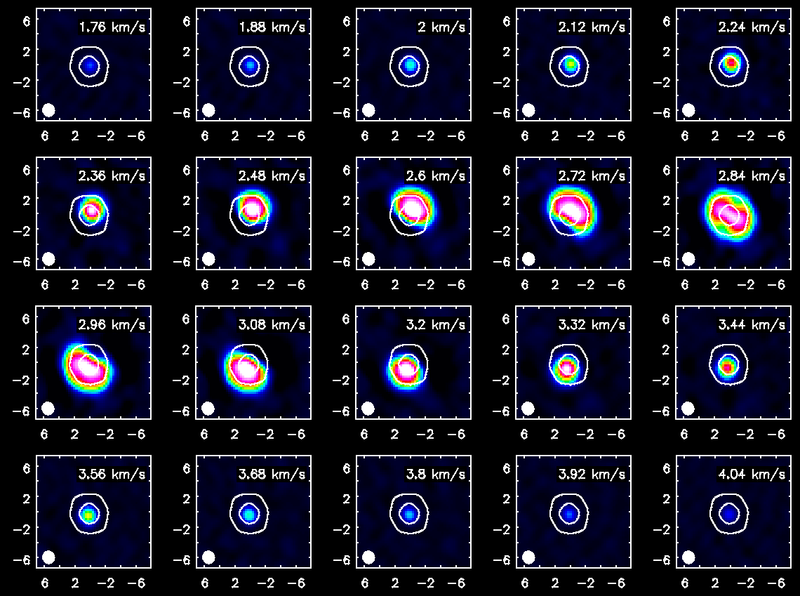
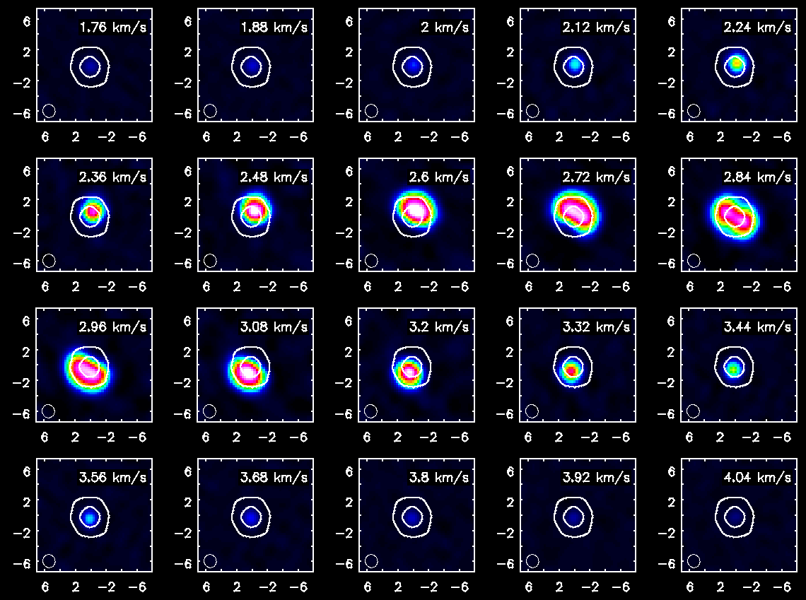
Display Channel Maps
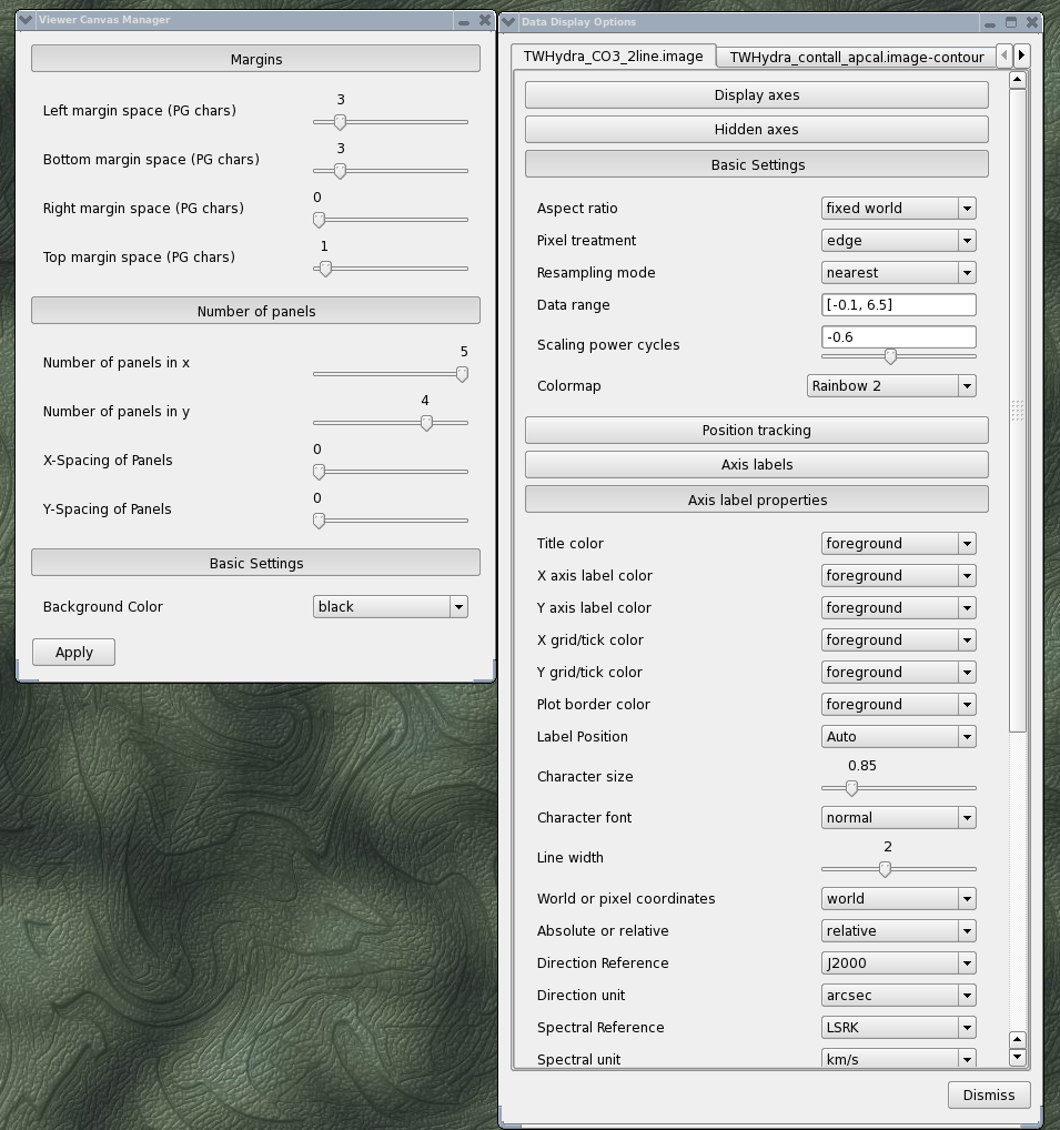
Using the Viewer you can make channel map figures. Start the Viewer and then open the CO(3-2) cube as a raster image and then the continuum as a contour image. Then we use the "wrench" icon and "P wrench" icons to set up the channel images, contour levels etc. (If you need help setting up the viewer for this image, see a screen shot of the viewer setup windows, below.)
<figure id="TWHya_channel_co3_2.png">
</figure>
<figure id="Viewer_setup.png">
</figure>
Repeat for HCO+(4-3)
<figure id="TWHya_channel_HCOp4_3.png">
</figure>
Last checked on CASA Version 4.5.0.
![The Data Display Panel used to set the color stretch, here from [-0.15, 0.15] with a linear (0) stretch. Setting the stretch to a negative value will highlight lower emission (a more logarithmic stretch). We got to this panel by clicking the wrench icon. You can also get from the dropdown menus (Data->Adjust).](/images/e/ed/DataDisplayPanelStretch.png)
