Guide To Processing ALMA Data for Cycle 0
Using the ALMA Data Archive for Cycle 0 Data
(rename the page with this title, when finished)
About this Guide, and Cycle 0 ALMA Data
This guide describes steps that you can use to process ALMA data, beginning with locating and downloading your data from the public archive, to making science-ready images.
We will use a sample data set from ALMA Cycle 0 in this guide. Data for Cycle 1 and beyond will be delivered in a different format and will require a separate guide.
For Cycle 0, ALMA data is delivered with a set of calibrated data files and a sample of reference images. The data were calibrated and imaged by an ALMA scientist at one of the ALMA Regional Centers (ARCs). The scientist developed CASA scripts that were used to complete the calibration and imaging. Cycle 0 data packages also include fully calibrated data sets, and the user can start with these data and proceed directly to imaging steps. In many cases, the imaging can be dramatically improved by including "self-calibration" steps. Self-calibration is the process of using the detected signal in the target source, itself, to tune the phase (and to a lesser extent, amplitude) calibrations, as a function of time.
The data package includes the calibration scripts used by the ARC scientist to perform the initial calibration and imaging steps. In most cases, users will not need to modify the calibration. But in some cases, some tuning of the calibration steps can improve the final images.
Typically, users interested in making science-ready images with Cycle 0 data from the ALMA archive will take the following steps:
- Download the data from the Archive
- Inspect the Quality Assurance plots and data files
- Inspect the reference images supplied with the data package
- Combine the calibrated data sets into a single calibrated measurement set
- Self-calibrate and image the combined data set
- Generate moment maps and other analysis products
Interested users may wish to review the calibration steps in detail, make modifications to the calibration script, and generate new calibrated data sets.
About the Sample Data: H2D+ and N2H+ in TW Hya
The data for this example comes from ALMA Project 2011.0.00340.S, "Searching for H2D+ in the disk of TW Hya v1.5", for which the PI is Chunhua Qi. Part of the data for this project has been published in Qi et al. 2013.
This observation has three scientific objectives:
- Image the submm continuum structure in TW Hya
- Image the H2D+ line structure (rest frequency 372.42138 GHz)
- Image the N2H+ line structure (rest frequency 372.67249 GHz)
Eventually we will see that the data is distilled to 4 "spectral windows" used for science. The N2H+ and H2D+ are each contained in one spectral window, and the other two windows contribute to the continuum observation. The best continuum map will be generated from the line-free channels of all 4 spectral windows.
Each spectral window covers 234.375 MHz in bandwidth, and the raw data contain 3840 channels, spaced by 61 kHz. Information on the spectral configuration and targets observed must be gleaned from the data themselves. In CASA, you can explore the contents of a data set using the listobs command.
What other data sets are available?
A Delivery List of publicly available data sets is provided on the ALMA Science Portal, in the "Data" tab.
Prerequisites : Computing Requirements
ALMA data sets can be very large and require significant computing resources for efficient processing. The data set used in this example begins with a download of 176 GB of data files. A description of recommended computing resources is given here. Those who do not have sufficient computing power may wish to arrange a visit to one of the ARCs to use the computing facilities at these sites. To arrange a visit to an ARC, submit a ticket to the ALMA Helpdesk.
Getting the Data: The ALMA Data Archive
The ALMA data archive is part of the ALMA Science Portal. A copy of the archive is stored at each of the ARCs, and you can connect to the nearest archive through these links:

|
| The ALMA Archive Query page. |
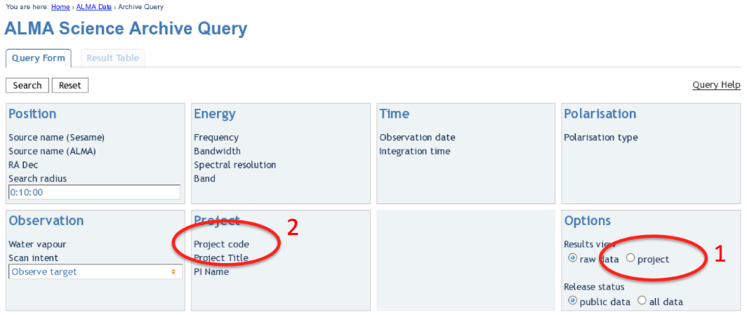
Upon entry into the ALMA Archive Query page, set the "Results View" option to "project" (see the red highlight #1 in the figure) and specify the Project Code to 2011.0.00340.S (red highlight #2). Note, if you leave the "Results View" set to "raw data", you will see three rows of data sets in the results page. These correspond to three executions of the observing script. In fact, cor Cycle 0 data these rows contains copies of the same data set, so use care not to download the (large!) data set three times. By setting "Results View" to project, you see just one entry, and that is the one you'd like to download.
You can download the data through the Archive GUI. For more control over the download process, you can use the Unix shell script provided on the Request Handler page. This script has a name like "downloadRequest84998259script.sh". You need to put this file into a directory that contains ample disk space, and execute is in you shell. For example, in bash:
# In bash
 % chmod +x downloadRequest84998259script.sh
 % ./downloadRequest84998259script.sh
Unpacking the data
The data you have downloaded includes 17 tar files. Unpack these using the following command:
# In bash
 % for i in $(ls *.tar); do echo 'Untarring ' $i; tar xvf $i; done
At this point you will have a directory called "2011.0.00340.S" with the full data distribution.
Overview of Delivered Data and Products
To get to the top-level directory that contains the data package, do:
# In bash
 % cd 2011.0.00340.S/sg_ouss_id/group_ouss_id/member_ouss_2012-12-05_id
Here you will find the following entries:
# In bash
 % ls
 calibrated  calibration  log  product  qa  raw  README  script
The README file describes the files in the distribution and includes notes from the ALMA scientist who performed the initial calibration and imaging.
The directories contain the following files:
-- calibrated/
  |-- uid___A002_X554543_X207.ms.split.cal/
  |-- uid___A002_X554543_X3d0.ms.split.cal/
  |-- uid___A002_X554543_X667.ms.split.cal/
-- calibration/
  |-- uid___A002_X554543_X207.calibration/
  |-- uid___A002_X554543_X207.calibration.plots/
  |-- uid___A002_X554543_X3d0.calibration/
  |-- uid___A002_X554543_X3d0.calibration.plots/
  |-- uid___A002_X554543_X667.calibration/
  |-- uid___A002_X554543_X667.calibration.plots/
-- log/
  |-- uid___A002_X554543_X207.calibration.log
  |-- uid___A002_X554543_X3d0.calibration.log
  |-- uid___A002_X554543_X667.calibration.log
  |-- Imaging.log
  |-- 340.log
-- product/
  |-- TWHya.continuum.fits
  |-- TWHya.N2H+.fits
  |-- TWHya.continuum.mask/
  |-- TWHya.H2D+.mask/
  |-- TWHya.N2H+.mask/
-- qa/
  |-- uid___A002_X554543_X207__textfile.txt
  |-- uid___A002_X554543_X207__qa2_part1.png
  |-- uid___A002_X554543_X207__qa2_part2.png
  |-- uid___A002_X554543_X207__qa2_part3.png
  |-- uid___A002_X554543_X3d0__textfile.txt
  |-- uid___A002_X554543_X3d0__qa2_part1.png
  |-- uid___A002_X554543_X3d0__qa2_part2.png
  |-- uid___A002_X554543_X3d0__qa2_part3.png
  |-- uid___A002_X554543_X667__textfile.txt
  |-- uid___A002_X554543_X667__qa2_part1.png
  |-- uid___A002_X554543_X667__qa2_part2.png
  |-- uid___A002_X554543_X667__qa2_part3.png
-- raw/
  |-- uid___A002_X554543_X207.ms.split/
  |-- uid___A002_X554543_X3d0.ms.split/
  |-- uid___A002_X554543_X667.ms.split/
-- script/
  |-- uid___A002_X554543_X207.ms.scriptForCalibration.py
  |-- uid___A002_X554543_X3d0.ms.scriptForCalibration.py
  |-- uid___A002_X554543_X667.ms.scriptForCalibration.py
  |-- scriptForImaging.py
  |-- import_data.py
  |-- scriptForFluxCalibration.py
- calibrated: This directory contains a calibrated measurement set for each of the three execution blocks. These could be imaged separately, or combined to make a single calibrated measurement set. In this guide we will combine these prior to imaging.
- calibration: Auxiliary data files generated in the calibration process.
- The "calibration.plots" directories contain (a few hundred) plots generated during the calibration process. These can be useful for the expert user to assess the quality of the calibration at each step.
- log: Describe here the data products and scripts. Pretty confused by these! See Scott Schnee.
- product: The final data products from the calibration and imaging process. The directory contains "reference" images that are used to determine the quality of the observation, but they are not necessarily science-ready. The data files here are useful for initial inspections.
- qa: The result of Quality Assessment tests. The data from each scheduling block goes through such a quality assessment, and all data delivered to the public ALMA Archive have passed the quality assessment. It is worthwhile to review the plots and text files contained here. You will find plots of the antenna configuration, UV coverage, calibration results, Tsys, and so on.
- raw: The "raw" data files. If you would like to tune or refine the calibration, these files would be your starting point. In fact, these data files do have certain a priori calibrations applied, amounting to steps 0-6 of the calibration scripts provided in the data package. These steps include a priori flagging and application of WVR, Tsys, and antenna position corrections.
- script: These are the scripts developed and applied by the ALMA scientist, to calibrate the data and generate reference images. These scripts cannot be applied directly to the raw data provided in this data distribution, but they can serve as a valuable reference to see the steps that need to be taken to reprocess the data, if you so choose.
What if I need to redo the Calibration?
In most cases, users should not need to re-do the calibration. However, you should consult this knowledgebase article for suggestions on when recalibration may be beneficial. If you do not need to redo calibration, proceed to Data Concatenation.
The data package includes a calibration script, for each execution of the scheduling block, that performs all the initial calibrations required prior to imaging the data set. The calibration script represents the exact step used to generate the packaged, calibrated data. However, for Cycle 0 data sets the script cannot be applied directly by the user. There are a couple of issues.
- The "raw" data supplied with the data package have had several a priori calibrations applied. These include calibration steps 0-6. So the user should begin with "step 7" in the packaged data reduction script.
- The data processing script was generated using CASA 3.4, but the users are recommended to use CASA 4.2 for all processing. There are a number of differences between these versions. The CASA 3.4 script should be used, therefore, as a guide to which steps need to be done, and in what order. But the script must be modified to work under CASA 4.2.
Updating a script to work with CASA 4.2
In the raw data directory are 3 measurement sets that are ready for calibration. [Here] are 3 calibration scripts updated to CASA 4.2, that can be used to calibrate these data sets. They can be run in CASA 4.2 as follows. (Start from the raw directory.)
# In CASA
 thesteps = [9,10,11,12,13,14,15,16,17,18,19]
 execfile('uid___A002_X554543_X207.ms.scriptForCalibration_4.2.py')
 execfile('uid___A002_X554543_X3d0.ms.scriptForCalibration_4.2.py')
 execfile('uid___A002_X554543_X667.ms.scriptForCalibration_4.2.py')
 execfile('scriptForFluxCalibration_4.2.py')
Flux Calibration
Prior to imaging, we must apply flux calibrations to the calibrated data sets, and then concatenate the three calibrated data sets into a single measurement set that we will then use for imaging. The script scriptForFluxCalibration.py will accomplish these tasks for us. If you copy that file into the raw data directory, you can then run it without modification, like so:
# In CASA
execfile('scriptForFluxCalibration.py')
If you would like to run each step by hand, you can follow the procedure [here].
Note, the scripts refers to the combined data set.
Data Concatenation
The data package includes a fully calibrated data set for each of the three execution blocks. To image the data, we start by combining the three data sets.
# In bash
 mkdir Imaging
 cd Imaging
 casapy
and then, in CASA:
# In CASA
concat(vis = ['../calibrated/uid___A002_X554543_X207.ms.split.cal', '../calibrated/uid___A002_X554543_X3d0.ms.split.cal',
       '../calibrated/uid___A002_X554543_X667.ms.split.cal'], concatvis = 'calibrated.ms')
This operation could take an hour or longer. When completed, we have created a calibrated measurement set calibrated.ms, which is ready for imaging.
Imaging
A first step is to list the contents of the calibarated.ms measurement set.
# In CASA
listobs(vis='calibrated.ms',listfile='calibrated.listobs')
The text file calibrated.listobs now contains a summary of the contents of this data file. The listobs output includes the following section:
Spectral Windows:  (4 unique spectral windows and 1 unique polarization setups)
 SpwID  Name                           #Chans   Frame   Ch0(MHz)  ChanWid(kHz)  TotBW(kHz) BBC Num  Corrs
 0      ALMA_RB_07#BB_1#SW-01#FULL_RES   3840   TOPO  372286.368        61.035    234375.0       1  XX  YY
 1      ALMA_RB_07#BB_2#SW-01#FULL_RES   3840   TOPO  372532.812        61.035    234375.0       2  XX  YY
 2      ALMA_RB_07#BB_3#SW-01#FULL_RES   3840   TOPO  358727.946       -61.035    234375.0       3  XX  YY
 3      ALMA_RB_07#BB_4#SW-01#FULL_RES   3840   TOPO  358040.598       -61.035    234375.0       4  XX  YY
We see that the data file contains 4 spectral windows. The H2D+ data are contained in SpwID=0 (rest frequency of H2D+: 372.42138) and the N2H+ data are contained in SpwID=1 (rest frequency of N2H+: 372.67249). Note that the Ch0 column gives the sky frequency at channel 0. To get central frequencies for the spectral windows, add 117.1875 MHz for Spectral Window IDs 0 and 1. Subtract 117.1875 MHz for IDs 2 and 3. (Note the channel width for these IDs is negative, indicating the frequencies increase in the opposite direction as SpwID 0 and 1.
Our strategy will be to image and self-calibrate the continuum data first. We will then apply the self-cal solutions to each of the two line data files, and image those second. In general terms, we will follow the steps outlines in the Science Verification CASAguide on TW Hya. You can also refer to the ScriptForImaging.py script included with the data package.
Continuum Imaging
First we will split off the TW Hya data and average the data over 100 channels, eliminating a few channels at each edge prior to averaging. This will generate a data set suitable for continuum imaging. The final data set has 6.1 MHz channels, sufficient to allow efficient cleaning with the "Multi-Frequency Synthesis" algorithm used by the CASA task clean.
# In CASA
split(vis='calibrated.ms', outputvis='TWHya_cont.ms', datacolumn='data', keepflags=T, field='TW Hya', spw='0~3:21~3820', width=100)
listobs(vis='TWHya_cont.ms', listfile='TWHya_cont.listobs')
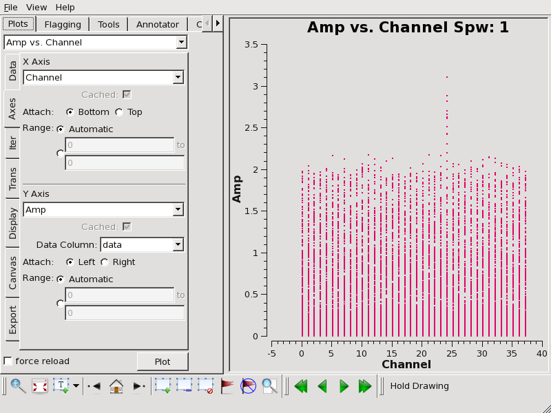
Now plot amplitude vs. channel with plotms to see what needs to be flagged.
# In CASA
plotms(vis='TWHya_cont.ms',spw='0~3',xaxis='channel',yaxis='amp',
      avgtime='1e8',avgscan=T,coloraxis='spw',iteraxis='spw',xselfscale=T)

|
| In SpwID = 1 we notice elevated amplitudes in channel 24. This arises from the strong N2H+ line emission. We'd like to flag this channel prior to imaging the continuum. |
We flag the line emission as follows:
# In CASA
flagdata(vis='TWHya_cont.ms', mode='manual', spw='1:24~24')
Next we will generate a first-pass continuum image. Note the mode "mfs" will generate a single continuum image from all the data.
# In CASA
os.system('rm -rf TWHya.continuum*')
clean(vis = 'TWHya_cont.ms',
  imagename = 'TWHya.continuum',
  field = '1', # TW Hya
  spw = '0~3',
  mode = 'mfs',
  imagermode = 'mosaic',
  interactive = T,
  imsize = [300, 300],
  cell = '0.1arcsec',
  phasecenter = 1,
  weighting = 'briggs',
  robust = 0.5)
Note that at ~370 GHz the ALMA primary beam has FWHM of ~ 20 arcseconds. We want to image an area at elast as large as that. Also, for this data set the synthesized beam is about 0.49 x 0.46 arcseconds. We have selected a cell size of 0.1 arcsec to fully sample the synthesized beam.
We'd like to do some cleaning to achieve our best image. In clean, the multifrequency synthesis mode grids each spectral channel independently. Since the uv-spacing is a function of frequency, this will actually achieve greater uv-coverage than if all the channels and spws had been averaged in advance.
Our initial cleaned model will be used as the image model in the next self-calibration step. It is essential that only "real" signal be included in the image model, so we will clean the image conservatively. We set interactive=T to make the clean mask interactively. This also allows us to stop clean when the signal from the source starts to approach the surrounding "noise" areas in the residual map.

|
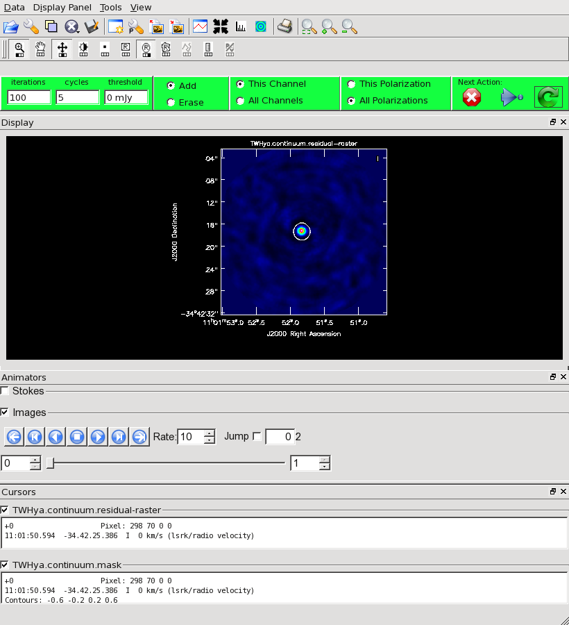
| After a few minutes, the clean procedure returns a plot of the dirty map as shown. |
Once the Clean Viewer opens, click on the ellipse tool with your left mouse button, and draw a circle around the continuum emission with the left mouse button. Double click inside the region with the left mouse button when you are happy with it. It will turn from green to white when the clean mask is accepted. To begin the clean use the green arrow in the "Next action" section on the Viewer Display GUI.
The red X will stop clean, the blue arrow will clean non-interactively
until reaching the number of iterations requested (niter) or the flux
density threshold (whichever comes first), and the green circle arrow
will clean until it reaches the "iterations" parameter on the left side
of the green area.
You should chose the green circle arrow. It will clean 100 iterations (as shown in the GUI) and then show the residual image. If necessary you can adjust the color scale to examine the residuals more clearly. The middle mouse button is initially assigned to the "plus" icon, which adjusts the colorscale. Also, note in the logger that clean reports the amount of clean flux recovered so far, the min/max residuals, and the synthesized beam.
We will clean 500 iterations by clicking the green arrow five times, without changing the clean mask. After this we have cleaned about 1.5 Jy and we have residuals of about 5-7 mJy.
There are a few points to note, with regard to the cleaning process:
- Real emission will not get "cleaned" if you do not put a clean box on it.
- Conversely, if you put a clean box on a region that contains no real emission and clean deeply, you can amplify that feature.
- Thus, it's best to be conservative. Stop cleaning when the residuals inside the clean box approach those outside it. Start with a small clean box surrounding what is clearly real emission, and add to it after some iterations, if necessary. You can generally see fainter "real" features in the residuals.
- If you start an interactive clean and then do not make a mask, the algorithm will clean nothing. There is no default mask.
clean will generate several files:
- TWHya.continuum.flux # the effective primary beam response (e.g. for pbcor)
- TWHya.continuum.flux.pbcoverage # the primary beam coverage (ftmachine=’mosaic’ only)
- TWHya.continuum.image # the final restored image
- TWHya.continuum.mask # the clean mask
- TWHya.continuum.model # the model image
- TWHya.continuum.psf # the synthesized (dirty) beam
- TWHya.continuum.residual # the residual image