M100 Band3 ACA 4.2.2
- This guide requires CASA 4.1.0 and assumes that you have downloaded M100_Band3_7m_CalibratedData.tgz from M100Band3#Obtaining_the_Data
- Details of the ALMA observations are provided at M100Band3
- This portion of the guide covers calibration of the raw visibility data. To skip to the imaging portion of the guide, see: M100Band3 Imaging 4.1.
Overview
This part of the M100 Band 3 7m CASA guide will step you through the calibration of the visibility data. We will begin by flagging (marking as bad) data known to be useless before any inspection, for example data where one telescope blocks the line of sight of another. Then we will apply telescope-generated calibration tables to partially correct for atmospheric effects. After inspecting the data, we will flag some additional data that exhibit pathologies. Then we will use observations of the calibrators Titan and 3c279 to derive the phase and amplitude response of individual antennas as a function of time and frequency ("phase", "amplitude", and "bandpass" calibrations). We will apply these to the data and then extract the calibrated source data into a file appropriate for imaging.
The general procedure in this guide follows the other ALMA CASA guides: NGC3256Band3 and TWHydraBand7.
Unpack the Data
Once you have downloaded the M100_Band3_7m_CalibratedData.tgz, unpack the file in a terminal outside CASA using
tar -xvzf M100_Band3_7m_CalibratedData.tgz
then change directory to the new directory
cd M100_Band3_7m_CalibratedData
You may wish to type
ls
to look at the files present. You should see a set of files with extension ".ms". These are CASA measurement set (MS) files. The data have already been converted to MS format from the native ALMA format using the CASA task importasdm. In addition to the data, we provide you with calibration tables containing system temperature (Tsys), water vapor radiometer (WVR), and antenna position information. For Early Science, these tables will either be pre-applied or supplied with the data.
This guide requires Python module analysisUtils. If you have not already installed analysisUtils please follow the link to do so.
To begin, start CASA by typing
casapy
Be sure that you are using the version indicated at the top of this page.
Confirm your version of CASA
This guide has been written for CASA release 4.1.0. Please confirm your version before proceeding.
# In CASA
version = casadef.casa_version
print "You are using " + version
if (version < '4.1.0'):
    print "YOUR VERSION OF CASA IS TOO OLD FOR THIS GUIDE."
    print "PLEASE UPDATE IT BEFORE PROCEEDING."
else:
    print "Your version of CASA is appropriate for this guide."
Install Analysis Utilities
Analysis Utilities (or analysisUtils for short) is a small set of Python scripts that provide a number of analysis and plotting utilities for ALMA data reduction. This guide uses a few of these utilities. They are very easy to install (just download and untar). See
http://casaguides.nrao.edu/index.php?title=Analysis_Utilities
for a full description and download instructions. Analysis Utilities are updated frequently so if its been a while since you installed it, its probably worth doing it again. If you are at an ALMA site or ARC, the analysis utilities are probably already installed and up to date.
Initial Inspection
First we will take stock of what we have. If you have not already done so, begin by reviewing the description of the observations here: M100Band3. The 6 data sets each target mosaic, as follows:
- uid___A002_X5e971a_X124.ms
- uid___A002_X5e971a_X2e7.ms
- uid___A002_X5e9ff1_X3f3.ms
- uid___A002_X5e9ff1_X5b3.ms
- uid___A002_X60b415_X44.ms
- uid___A002_X62f759_X4eb.ms
The first step is to get basic information about the data: targets observed, time range, spectral setup, and so on. We do this using the task listobs, which will output a detailed summary of each dataset. Enter the following commands into CASA:
# In CASA

# Define a python list holding the names of all of our data sets
basename=['uid___A002_X5e971a_X124','uid___A002_X5e971a_X2e7','uid___A002_X5e9ff1_X3f3','uid___A002_X5e9ff1_X5b3', 'uid___A002_X60b415_X44','uid___A002_X62f759_X4eb']

# Initialize user-input string.  (for Python testing)
dummy_string = ''

# Loop over each element in the list and create summary file using listobs
for asdm in basename_all:
    os.system('rm '+asdm+'.listobs.txt')
    listobs(vis=asdm+'.ms', listfile=asdm+'.listobs.txt', verbose=True)
Note that after cutting and pasting a 'for' loop like this you often have to press return twice to execute. You may also want to take care to paste a line at a time if you are having trouble copy and pasting. Even better, you can use "cpaste" to paste blocks of code. To do so type "cpaste" at the CASA prompt, paste your commands, and then type "--" and hit return on the final (otherwise empty) line. This should look something like this:
CASA <8>: cpaste
Pasting code; enter '--' alone on the line to stop.
:basename=['uid___A002_X5e971a_X124','uid___A002_X5e971a_X2e7','uid___A002_X5e9ff1_X3f3','uid___A002_X5e9ff1_X5b3', 'uid___A002_X60b415_X44','uid___A002_X62f759_X4eb']
:
:for asdm in basename_all:
:    print asdm
:--
uid___A002_X5e971a_X124
uid___A002_X5e971a_X2e7
uid___A002_X5e9ff1_X3f3
uid___A002_X5e9ff1_X5b3
uid___A002_X60b415_X44
uid___A002_X62f759_X4eb

CASA <9>:
cpaste should be much more robust than copying-and-pasting directly into the shell but if you have trouble, just carefully paste one line at a time directly into CASA and hit return until the desired command executes.
These commands define a python list called "basename_all", which contains the name of all 6 MS files. The "for" loop executes for each element in basename_all, calling listobs and directing the output to a file called, e.g., "uid___A002_X5e971a_X124.ms.listobs.txt" for the first measurement set. You can browse through the listobs output as you would normally look at a text file (use emacs, vi, or another editor). You can also send the output to the terminal from inside of CASA. To do so type:
# In CASA
os.system('cat uid___A002_X5e971a_X124.ms.listobs.txt')
or
# In CASA
os.system('more uid___A002_X5e971a_X124.ms.listobs.txt')
CASA knows a few basic shell commands like 'cat', 'ls', and 'rm' but for more complex commands you will need to run them inside 'os.system("command")'. For more information see http://casa.nrao.edu/ .
Here is an example of the (abridged) output from listobs for the first dataset in the list, uid___A002_X5e971a_X124.ms, which targets the Northern Mosaic. You would see this if you had specified verbose to be False in the listobs call:
================================================================================
MeasurementSet Name: /lustre/naasc/almauser/M100Band3/uid___A002_X5e971a_X124.ms MS Version 2
================================================================================
Observer: cvlahakis Project: uid://A002/X5d9e5c/X5d
Observation: ALMA
Data records: 940680 Total integration time = 5436.77 seconds
Observed from 17-Mar-2013/04:07:32.8 to 17-Mar-2013/05:38:09.6 (UTC)
ObservationID = 0 ArrayID = 0
Date Timerange (UTC) Scan FldId FieldName nRows nUnflRows SpwIds Average Interval(s) ScanIntent
17-Mar-2013/04:07:32.3 - 04:09:35.4 1 0 J1229+0203 43200 43200.00 [0, 1, 2, 3, 4, 5, 6, 7] [1.01, 1.01, 1.01, 1.01, 1.01, 1.01, 1.01, 1.01] CALIBRATE_POINTING#ON_SOURCE
04:10:57.2 - 04:11:57.7 2 0 J1229+0203 45360 45360.00 [8, 9, 10, 11, 12, 13, 14, 15] [0.48, 0.48, 0.48, 0.48, 0.48, 0.48, 0.48, 0.48] CALIBRATE_SIDEBAND_RATIO#ON_SOURCE
04:12:48.5 - 04:14:00.0 3 0 J1229+0203 12960 12960.00 [8, 9, 10, 11, 12, 13, 14, 15] [0.48, 0.48, 0.48, 0.48, 0.48, 0.48, 0.48, 0.48] CALIBRATE_ATMOSPHERE#ON_SOURCE
04:14:44.2 - 04:24:49.9 4 0 J1229+0203 118800 44880.00 [16, 17, 18, 19, 20, 21, 22, 23] [10.1, 1.01, 10.1, 1.01, 10.1, 1.01, 10.1, 1.01] CALIBRATE_BANDPASS#ON_SOURCE
04:25:53.4 - 04:27:56.4 5 1 J1445-1629 43200 43200.00 [0, 1, 2, 3, 4, 5, 6, 7] [1.01, 1.01, 1.01, 1.01, 1.01, 1.01, 1.01, 1.01] CALIBRATE_POINTING#ON_SOURCE
04:29:02.6 - 04:30:13.9 6 2 Titan 12960 12960.00 [8, 9, 10, 11, 12, 13, 14, 15] [0.48, 0.48, 0.48, 0.48, 0.48, 0.48, 0.48, 0.48] CALIBRATE_ATMOSPHERE#ON_SOURCE
04:30:57.7 - 04:36:00.5 7 2 Titan 59400 22468.00 [16, 17, 18, 19, 20, 21, 22, 23] [10.1, 1.01, 10.1, 1.01, 10.1, 1.01, 10.1, 1.01] CALIBRATE_AMPLI#ON_SOURCE
04:37:10.1 - 04:39:13.2 8 3 J1215+1654 43200 43200.00 [0, 1, 2, 3, 4, 5, 6, 7] [1.01, 1.01, 1.01, 1.01, 1.01, 1.01, 1.01, 1.01] CALIBRATE_POINTING#ON_SOURCE
04:39:58.8 - 04:40:59.3 9 3 J1215+1654 11880 4488.00 [16, 17, 18, 19, 20, 21, 22, 23] [10.1, 1.01, 10.1, 1.01, 10.1, 1.01, 10.1, 1.01] CALIBRATE_PHASE#ON_SOURCE
04:42:08.6 - 04:43:20.0 10 4 M100 12960 12960.00 [8, 9, 10, 11, 12, 13, 14, 15] [0.48, 0.48, 0.48, 0.48, 0.48, 0.48, 0.48, 0.48] CALIBRATE_ATMOSPHERE#ON_SOURCE
04:44:04.3 - 04:50:43.7 11 5 M100 5940 2244.00 [16, 17, 18, 19, 20, 21, 22, 23] [10.1, 1.01, 10.1, 1.01, 10.1, 1.01, 10.1, 1.01] OBSERVE_TARGET#ON_SOURCE
04:44:04.3 - 04:50:43.7 11 6 M100 5940 2244.00 [16, 17, 18, 19, 20, 21, 22, 23] [10.1, 1.01, 10.1, 1.01, 10.1, 1.01, 10.1, 1.01] OBSERVE_TARGET#ON_SOURCE
04:44:04.3 - 04:50:43.7 11 7 M100 5940 2244.00 [16, 17, 18, 19, 20, 21, 22, 23] [10.1, 1.01, 10.1, 1.01, 10.1, 1.01, 10.1, 1.01] OBSERVE_TARGET#ON_SOURCE
04:44:04.3 - 04:50:43.7 11 8 M100 5940 2244.00 [16, 17, 18, 19, 20, 21, 22, 23] [10.1, 1.01, 10.1, 1.01, 10.1, 1.01, 10.1, 1.01] OBSERVE_TARGET#ON_SOURCE
04:44:04.3 - 04:50:43.7 11 9 M100 5940 2244.00 [16, 17, 18, 19, 20, 21, 22, 23] [10.1, 1.01, 10.1, 1.01, 10.1, 1.01, 10.1, 1.01] OBSERVE_TARGET#ON_SOURCE
04:44:04.3 - 04:50:43.7 11 10 M100 5940 2244.00 [16, 17, 18, 19, 20, 21, 22, 23] [10.1, 1.01, 10.1, 1.01, 10.1, 1.01, 10.1, 1.01] OBSERVE_TARGET#ON_SOURCE
04:44:04.3 - 04:50:43.7 11 11 M100 5940 2244.00 [16, 17, 18, 19, 20, 21, 22, 23] [10.1, 1.01, 10.1, 1.01, 10.1, 1.01, 10.1, 1.01] OBSERVE_TARGET#ON_SOURCE
04:44:04.3 - 04:50:43.7 11 12 M100 5940 2244.00 [16, 17, 18, 19, 20, 21, 22, 23] [10.1, 1.01, 10.1, 1.01, 10.1, 1.01, 10.1, 1.01] OBSERVE_TARGET#ON_SOURCE
04:44:04.3 - 04:50:43.7 11 13 M100 5940 2244.00 [16, 17, 18, 19, 20, 21, 22, 23] [10.1, 1.01, 10.1, 1.01, 10.1, 1.01, 10.1, 1.01] OBSERVE_TARGET#ON_SOURCE
04:44:04.3 - 04:50:43.7 11 14 M100 5940 2244.00 [16, 17, 18, 19, 20, 21, 22, 23] [10.1, 1.01, 10.1, 1.01, 10.1, 1.01, 10.1, 1.01] OBSERVE_TARGET#ON_SOURCE
04:44:04.3 - 04:50:43.7 11 15 M100 5940 2244.00 [16, 17, 18, 19, 20, 21, 22, 23] [10.1, 1.01, 10.1, 1.01, 10.1, 1.01, 10.1, 1.01] OBSERVE_TARGET#ON_SOURCE
04:44:04.3 - 04:50:43.7 11 16 M100 5940 2244.00 [16, 17, 18, 19, 20, 21, 22, 23] [10.1, 1.01, 10.1, 1.01, 10.1, 1.01, 10.1, 1.01] OBSERVE_TARGET#ON_SOURCE
04:44:04.3 - 04:50:43.7 11 17 M100 5940 2244.00 [16, 17, 18, 19, 20, 21, 22, 23] [10.1, 1.01, 10.1, 1.01, 10.1, 1.01, 10.1, 1.01] OBSERVE_TARGET#ON_SOURCE
04:51:04.3 - 04:52:04.8 12 3 J1215+1654 11880 4488.00 [16, 17, 18, 19, 20, 21, 22, 23] [10.1, 1.01, 10.1, 1.01, 10.1, 1.01, 10.1, 1.01] CALIBRATE_PHASE#ON_SOURCE
04:52:35.8 - 04:59:15.3 13 5 M100 5940 2244.00 [16, 17, 18, 19, 20, 21, 22, 23] [10.1, 1.01, 10.1, 1.01, 10.1, 1.01, 10.1, 1.01] OBSERVE_TARGET#ON_SOURCE
04:52:35.8 - 04:59:15.3 13 6 M100 5940 2244.00 [16, 17, 18, 19, 20, 21, 22, 23] [10.1, 1.01, 10.1, 1.01, 10.1, 1.01, 10.1, 1.01] OBSERVE_TARGET#ON_SOURCE
04:52:35.8 - 04:59:15.3 13 7 M100 5940 2244.00 [16, 17, 18, 19, 20, 21, 22, 23] [10.1, 1.01, 10.1, 1.01, 10.1, 1.01, 10.1, 1.01] OBSERVE_TARGET#ON_SOURCE
04:52:35.8 - 04:59:15.3 13 18 M100 5940 2244.00 [16, 17, 18, 19, 20, 21, 22, 23] [10.1, 1.01, 10.1, 1.01, 10.1, 1.01, 10.1, 1.01] OBSERVE_TARGET#ON_SOURCE
04:52:35.8 - 04:59:15.3 13 19 M100 5940 2244.00 [16, 17, 18, 19, 20, 21, 22, 23] [10.1, 1.01, 10.1, 1.01, 10.1, 1.01, 10.1, 1.01] OBSERVE_TARGET#ON_SOURCE
04:52:35.8 - 04:59:15.3 13 20 M100 5940 2244.00 [16, 17, 18, 19, 20, 21, 22, 23] [10.1, 1.01, 10.1, 1.01, 10.1, 1.01, 10.1, 1.01] OBSERVE_TARGET#ON_SOURCE
04:52:35.8 - 04:59:15.3 13 21 M100 5940 2244.00 [16, 17, 18, 19, 20, 21, 22, 23] [10.1, 1.01, 10.1, 1.01, 10.1, 1.01, 10.1, 1.01] OBSERVE_TARGET#ON_SOURCE
04:52:35.8 - 04:59:15.3 13 22 M100 5940 2244.00 [16, 17, 18, 19, 20, 21, 22, 23] [10.1, 1.01, 10.1, 1.01, 10.1, 1.01, 10.1, 1.01] OBSERVE_TARGET#ON_SOURCE
04:52:35.8 - 04:59:15.3 13 23 M100 5940 2244.00 [16, 17, 18, 19, 20, 21, 22, 23] [10.1, 1.01, 10.1, 1.01, 10.1, 1.01, 10.1, 1.01] OBSERVE_TARGET#ON_SOURCE
04:52:35.8 - 04:59:15.3 13 24 M100 5940 2244.00 [16, 17, 18, 19, 20, 21, 22, 23] [10.1, 1.01, 10.1, 1.01, 10.1, 1.01, 10.1, 1.01] OBSERVE_TARGET#ON_SOURCE
04:52:35.8 - 04:59:15.3 13 25 M100 5940 2244.00 [16, 17, 18, 19, 20, 21, 22, 23] [10.1, 1.01, 10.1, 1.01, 10.1, 1.01, 10.1, 1.01] OBSERVE_TARGET#ON_SOURCE
04:52:35.8 - 04:59:15.3 13 26 M100 5940 2244.00 [16, 17, 18, 19, 20, 21, 22, 23] [10.1, 1.01, 10.1, 1.01, 10.1, 1.01, 10.1, 1.01] OBSERVE_TARGET#ON_SOURCE
04:52:35.8 - 04:59:15.3 13 27 M100 5940 2244.00 [16, 17, 18, 19, 20, 21, 22, 23] [10.1, 1.01, 10.1, 1.01, 10.1, 1.01, 10.1, 1.01] OBSERVE_TARGET#ON_SOURCE
04:59:35.7 - 05:00:36.2 14 3 J1215+1654 11880 4488.00 [16, 17, 18, 19, 20, 21, 22, 23] [10.1, 1.01, 10.1, 1.01, 10.1, 1.01, 10.1, 1.01] CALIBRATE_PHASE#ON_SOURCE
05:01:55.1 - 05:03:06.5 15 4 M100 12960 12960.00 [8, 9, 10, 11, 12, 13, 14, 15] [0.48, 0.48, 0.48, 0.48, 0.48, 0.48, 0.48, 0.48] CALIBRATE_ATMOSPHERE#ON_SOURCE
05:03:22.2 - 05:10:01.6 16 8 M100 5940 2244.00 [16, 17, 18, 19, 20, 21, 22, 23] [10.1, 1.01, 10.1, 1.01, 10.1, 1.01, 10.1, 1.01] OBSERVE_TARGET#ON_SOURCE
05:03:22.2 - 05:10:01.6 16 9 M100 5940 2244.00 [16, 17, 18, 19, 20, 21, 22, 23] [10.1, 1.01, 10.1, 1.01, 10.1, 1.01, 10.1, 1.01] OBSERVE_TARGET#ON_SOURCE
05:03:22.2 - 05:10:01.6 16 10 M100 5940 2244.00 [16, 17, 18, 19, 20, 21, 22, 23] [10.1, 1.01, 10.1, 1.01, 10.1, 1.01, 10.1, 1.01] OBSERVE_TARGET#ON_SOURCE
05:03:22.2 - 05:10:01.6 16 11 M100 5940 2244.00 [16, 17, 18, 19, 20, 21, 22, 23] [10.1, 1.01, 10.1, 1.01, 10.1, 1.01, 10.1, 1.01] OBSERVE_TARGET#ON_SOURCE
05:03:22.2 - 05:10:01.6 16 12 M100 5940 2244.00 [16, 17, 18, 19, 20, 21, 22, 23] [10.1, 1.01, 10.1, 1.01, 10.1, 1.01, 10.1, 1.01] OBSERVE_TARGET#ON_SOURCE
05:03:22.2 - 05:10:01.6 16 13 M100 5940 2244.00 [16, 17, 18, 19, 20, 21, 22, 23] [10.1, 1.01, 10.1, 1.01, 10.1, 1.01, 10.1, 1.01] OBSERVE_TARGET#ON_SOURCE
05:03:22.2 - 05:10:01.6 16 14 M100 5940 2244.00 [16, 17, 18, 19, 20, 21, 22, 23] [10.1, 1.01, 10.1, 1.01, 10.1, 1.01, 10.1, 1.01] OBSERVE_TARGET#ON_SOURCE
05:03:22.2 - 05:10:01.6 16 15 M100 5940 2244.00 [16, 17, 18, 19, 20, 21, 22, 23] [10.1, 1.01, 10.1, 1.01, 10.1, 1.01, 10.1, 1.01] OBSERVE_TARGET#ON_SOURCE
05:03:22.2 - 05:10:01.6 16 16 M100 5940 2244.00 [16, 17, 18, 19, 20, 21, 22, 23] [10.1, 1.01, 10.1, 1.01, 10.1, 1.01, 10.1, 1.01] OBSERVE_TARGET#ON_SOURCE
05:03:22.2 - 05:10:01.6 16 17 M100 5940 2244.00 [16, 17, 18, 19, 20, 21, 22, 23] [10.1, 1.01, 10.1, 1.01, 10.1, 1.01, 10.1, 1.01] OBSERVE_TARGET#ON_SOURCE
05:03:22.2 - 05:10:01.6 16 18 M100 5940 2244.00 [16, 17, 18, 19, 20, 21, 22, 23] [10.1, 1.01, 10.1, 1.01, 10.1, 1.01, 10.1, 1.01] OBSERVE_TARGET#ON_SOURCE
05:03:22.2 - 05:10:01.6 16 19 M100 5940 2244.00 [16, 17, 18, 19, 20, 21, 22, 23] [10.1, 1.01, 10.1, 1.01, 10.1, 1.01, 10.1, 1.01] OBSERVE_TARGET#ON_SOURCE
05:03:22.2 - 05:10:01.6 16 20 M100 5940 2244.00 [16, 17, 18, 19, 20, 21, 22, 23] [10.1, 1.01, 10.1, 1.01, 10.1, 1.01, 10.1, 1.01] OBSERVE_TARGET#ON_SOURCE
05:10:50.7 - 05:11:51.2 17 3 J1215+1654 11880 4488.00 [16, 17, 18, 19, 20, 21, 22, 23] [10.1, 1.01, 10.1, 1.01, 10.1, 1.01, 10.1, 1.01] CALIBRATE_PHASE#ON_SOURCE
05:12:22.0 - 05:19:01.4 18 5 M100 5940 2244.00 [16, 17, 18, 19, 20, 21, 22, 23] [10.1, 1.01, 10.1, 1.01, 10.1, 1.01, 10.1, 1.01] OBSERVE_TARGET#ON_SOURCE
05:12:22.0 - 05:19:01.4 18 6 M100 5940 2244.00 [16, 17, 18, 19, 20, 21, 22, 23] [10.1, 1.01, 10.1, 1.01, 10.1, 1.01, 10.1, 1.01] OBSERVE_TARGET#ON_SOURCE
05:12:22.0 - 05:19:01.4 18 7 M100 5940 2244.00 [16, 17, 18, 19, 20, 21, 22, 23] [10.1, 1.01, 10.1, 1.01, 10.1, 1.01, 10.1, 1.01] OBSERVE_TARGET#ON_SOURCE
05:12:22.0 - 05:19:01.4 18 8 M100 5940 2244.00 [16, 17, 18, 19, 20, 21, 22, 23] [10.1, 1.01, 10.1, 1.01, 10.1, 1.01, 10.1, 1.01] OBSERVE_TARGET#ON_SOURCE
05:12:22.0 - 05:19:01.4 18 9 M100 5940 2244.00 [16, 17, 18, 19, 20, 21, 22, 23] [10.1, 1.01, 10.1, 1.01, 10.1, 1.01, 10.1, 1.01] OBSERVE_TARGET#ON_SOURCE
05:12:22.0 - 05:19:01.4 18 10 M100 5940 2244.00 [16, 17, 18, 19, 20, 21, 22, 23] [10.1, 1.01, 10.1, 1.01, 10.1, 1.01, 10.1, 1.01] OBSERVE_TARGET#ON_SOURCE
05:12:22.0 - 05:19:01.4 18 21 M100 5940 2244.00 [16, 17, 18, 19, 20, 21, 22, 23] [10.1, 1.01, 10.1, 1.01, 10.1, 1.01, 10.1, 1.01] OBSERVE_TARGET#ON_SOURCE
05:12:22.0 - 05:19:01.4 18 22 M100 5940 2244.00 [16, 17, 18, 19, 20, 21, 22, 23] [10.1, 1.01, 10.1, 1.01, 10.1, 1.01, 10.1, 1.01] OBSERVE_TARGET#ON_SOURCE
05:12:22.0 - 05:19:01.4 18 23 M100 5940 2244.00 [16, 17, 18, 19, 20, 21, 22, 23] [10.1, 1.01, 10.1, 1.01, 10.1, 1.01, 10.1, 1.01] OBSERVE_TARGET#ON_SOURCE
05:12:22.0 - 05:19:01.4 18 24 M100 5940 2244.00 [16, 17, 18, 19, 20, 21, 22, 23] [10.1, 1.01, 10.1, 1.01, 10.1, 1.01, 10.1, 1.01] OBSERVE_TARGET#ON_SOURCE
05:12:22.0 - 05:19:01.4 18 25 M100 5940 2244.00 [16, 17, 18, 19, 20, 21, 22, 23] [10.1, 1.01, 10.1, 1.01, 10.1, 1.01, 10.1, 1.01] OBSERVE_TARGET#ON_SOURCE
05:12:22.0 - 05:19:01.4 18 26 M100 5940 2244.00 [16, 17, 18, 19, 20, 21, 22, 23] [10.1, 1.01, 10.1, 1.01, 10.1, 1.01, 10.1, 1.01] OBSERVE_TARGET#ON_SOURCE
05:12:22.0 - 05:19:01.4 18 27 M100 5940 2244.00 [16, 17, 18, 19, 20, 21, 22, 23] [10.1, 1.01, 10.1, 1.01, 10.1, 1.01, 10.1, 1.01] OBSERVE_TARGET#ON_SOURCE
05:19:22.0 - 05:20:22.6 19 3 J1215+1654 11880 4488.00 [16, 17, 18, 19, 20, 21, 22, 23] [10.1, 1.01, 10.1, 1.01, 10.1, 1.01, 10.1, 1.01] CALIBRATE_PHASE#ON_SOURCE
05:21:41.7 - 05:22:53.4 20 4 M100 12960 12960.00 [8, 9, 10, 11, 12, 13, 14, 15] [0.48, 0.48, 0.48, 0.48, 0.48, 0.48, 0.48, 0.48] CALIBRATE_ATMOSPHERE#ON_SOURCE
05:23:37.6 - 05:30:17.0 21 11 M100 5940 2244.00 [16, 17, 18, 19, 20, 21, 22, 23] [10.1, 1.01, 10.1, 1.01, 10.1, 1.01, 10.1, 1.01] OBSERVE_TARGET#ON_SOURCE
05:23:37.6 - 05:30:17.0 21 12 M100 5940 2244.00 [16, 17, 18, 19, 20, 21, 22, 23] [10.1, 1.01, 10.1, 1.01, 10.1, 1.01, 10.1, 1.01] OBSERVE_TARGET#ON_SOURCE
05:23:37.6 - 05:30:17.0 21 13 M100 5940 2244.00 [16, 17, 18, 19, 20, 21, 22, 23] [10.1, 1.01, 10.1, 1.01, 10.1, 1.01, 10.1, 1.01] OBSERVE_TARGET#ON_SOURCE
05:23:37.6 - 05:30:17.0 21 14 M100 5940 2244.00 [16, 17, 18, 19, 20, 21, 22, 23] [10.1, 1.01, 10.1, 1.01, 10.1, 1.01, 10.1, 1.01] OBSERVE_TARGET#ON_SOURCE
05:23:37.6 - 05:30:17.0 21 15 M100 5940 2244.00 [16, 17, 18, 19, 20, 21, 22, 23] [10.1, 1.01, 10.1, 1.01, 10.1, 1.01, 10.1, 1.01] OBSERVE_TARGET#ON_SOURCE
05:23:37.6 - 05:30:17.0 21 16 M100 5940 2244.00 [16, 17, 18, 19, 20, 21, 22, 23] [10.1, 1.01, 10.1, 1.01, 10.1, 1.01, 10.1, 1.01] OBSERVE_TARGET#ON_SOURCE
05:23:37.6 - 05:30:17.0 21 17 M100 5940 2244.00 [16, 17, 18, 19, 20, 21, 22, 23] [10.1, 1.01, 10.1, 1.01, 10.1, 1.01, 10.1, 1.01] OBSERVE_TARGET#ON_SOURCE
05:23:37.6 - 05:30:17.0 21 18 M100 5940 2244.00 [16, 17, 18, 19, 20, 21, 22, 23] [10.1, 1.01, 10.1, 1.01, 10.1, 1.01, 10.1, 1.01] OBSERVE_TARGET#ON_SOURCE
05:23:37.6 - 05:30:17.0 21 19 M100 5940 2244.00 [16, 17, 18, 19, 20, 21, 22, 23] [10.1, 1.01, 10.1, 1.01, 10.1, 1.01, 10.1, 1.01] OBSERVE_TARGET#ON_SOURCE
05:23:37.6 - 05:30:17.0 21 20 M100 5940 2244.00 [16, 17, 18, 19, 20, 21, 22, 23] [10.1, 1.01, 10.1, 1.01, 10.1, 1.01, 10.1, 1.01] OBSERVE_TARGET#ON_SOURCE
05:23:37.6 - 05:30:17.0 21 21 M100 5940 2244.00 [16, 17, 18, 19, 20, 21, 22, 23] [10.1, 1.01, 10.1, 1.01, 10.1, 1.01, 10.1, 1.01] OBSERVE_TARGET#ON_SOURCE
05:23:37.6 - 05:30:17.0 21 22 M100 5940 2244.00 [16, 17, 18, 19, 20, 21, 22, 23] [10.1, 1.01, 10.1, 1.01, 10.1, 1.01, 10.1, 1.01] OBSERVE_TARGET#ON_SOURCE
05:23:37.6 - 05:30:17.0 21 23 M100 5940 2244.00 [16, 17, 18, 19, 20, 21, 22, 23] [10.1, 1.01, 10.1, 1.01, 10.1, 1.01, 10.1, 1.01] OBSERVE_TARGET#ON_SOURCE
05:30:37.5 - 05:31:38.1 22 3 J1215+1654 11880 4488.00 [16, 17, 18, 19, 20, 21, 22, 23] [10.1, 1.01, 10.1, 1.01, 10.1, 1.01, 10.1, 1.01] CALIBRATE_PHASE#ON_SOURCE
05:32:08.4 - 05:36:44.7 23 5 M100 5940 2244.00 [16, 17, 18, 19, 20, 21, 22, 23] [10.1, 1.01, 10.1, 1.01, 10.1, 1.01, 10.1, 1.01] OBSERVE_TARGET#ON_SOURCE
05:32:08.4 - 05:36:44.7 23 6 M100 5940 2244.00 [16, 17, 18, 19, 20, 21, 22, 23] [10.1, 1.01, 10.1, 1.01, 10.1, 1.01, 10.1, 1.01] OBSERVE_TARGET#ON_SOURCE
05:32:08.4 - 05:36:44.7 23 7 M100 5940 2244.00 [16, 17, 18, 19, 20, 21, 22, 23] [10.1, 1.01, 10.1, 1.01, 10.1, 1.01, 10.1, 1.01] OBSERVE_TARGET#ON_SOURCE
05:32:08.4 - 05:36:44.7 23 8 M100 5940 2244.00 [16, 17, 18, 19, 20, 21, 22, 23] [10.1, 1.01, 10.1, 1.01, 10.1, 1.01, 10.1, 1.01] OBSERVE_TARGET#ON_SOURCE
05:32:08.4 - 05:36:44.7 23 9 M100 5940 2244.00 [16, 17, 18, 19, 20, 21, 22, 23] [10.1, 1.01, 10.1, 1.01, 10.1, 1.01, 10.1, 1.01] OBSERVE_TARGET#ON_SOURCE
05:32:08.4 - 05:36:44.7 23 24 M100 5940 2244.00 [16, 17, 18, 19, 20, 21, 22, 23] [10.1, 1.01, 10.1, 1.01, 10.1, 1.01, 10.1, 1.01] OBSERVE_TARGET#ON_SOURCE
05:32:08.4 - 05:36:44.7 23 25 M100 5940 2244.00 [16, 17, 18, 19, 20, 21, 22, 23] [10.1, 1.01, 10.1, 1.01, 10.1, 1.01, 10.1, 1.01] OBSERVE_TARGET#ON_SOURCE
05:32:08.4 - 05:36:44.7 23 26 M100 5940 2244.00 [16, 17, 18, 19, 20, 21, 22, 23] [10.1, 1.01, 10.1, 1.01, 10.1, 1.01, 10.1, 1.01] OBSERVE_TARGET#ON_SOURCE
05:32:08.4 - 05:36:44.7 23 27 M100 5940 2244.00 [16, 17, 18, 19, 20, 21, 22, 23] [10.1, 1.01, 10.1, 1.01, 10.1, 1.01, 10.1, 1.01] OBSERVE_TARGET#ON_SOURCE
05:37:09.6 - 05:38:10.1 24 3 J1215+1654 11880 4488.00 [16, 17, 18, 19, 20, 21, 22, 23] [10.1, 1.01, 10.1, 1.01, 10.1, 1.01, 10.1, 1.01] CALIBRATE_PHASE#ON_SOURCE
(nRows = Total number of rows per scan)
Fields: 28
ID Code Name RA Decl Epoch SrcId nRows nUnflRows
0 none J1229+0203 12:29:06.699720 +02.03.08.59820 J2000 0 220320 146400.00
1 none J1445-1629 14:45:53.376290 -16.29.01.61880 J2000 1 43200 43200.00
2 none Titan 14:36:50.919019 -12.33.38.18202 J2000 1 72360 35428.00
3 none J1215+1654 12:15:03.979130 +16.54.37.95700 J2000 2 126360 74616.00
4 none M100 12:22:54.899040 +15.49.20.57160 J2000 2 38880 38880.00
5 none M100 12:22:57.009007 +15.49.13.60358 J2000 3 23760 8976.00
6 none M100 12:22:57.009041 +15.49.58.08112 J2000 3 23760 8976.00
7 none M100 12:22:54.339884 +15.47.22.41016 J2000 3 23760 8976.00
8 none M100 12:22:54.339918 +15.48.06.88770 J2000 3 23760 8976.00
9 none M100 12:22:54.339952 +15.48.51.36524 J2000 3 23760 8976.00
10 none M100 12:22:54.339986 +15.49.35.84278 J2000 3 17820 6732.00
11 none M100 12:22:54.340020 +15.50.20.32032 J2000 3 17820 6732.00
12 none M100 12:22:51.670863 +15.47.44.64936 J2000 3 17820 6732.00
13 none M100 12:22:51.670897 +15.48.29.12690 J2000 3 17820 6732.00
14 none M100 12:22:51.670931 +15.49.13.60444 J2000 3 17820 6732.00
15 none M100 12:22:51.670966 +15.49.58.08198 J2000 3 17820 6732.00
16 none M100 12:22:49.001808 +15.47.22.41102 J2000 3 17820 6732.00
17 none M100 12:22:49.001842 +15.48.06.88856 J2000 3 17820 6732.00
18 none M100 12:22:49.001876 +15.48.51.36610 J2000 3 17820 6732.00
19 none M100 12:22:49.001911 +15.49.35.84364 J2000 3 17820 6732.00
20 none M100 12:22:49.001945 +15.50.20.32118 J2000 3 17820 6732.00
21 none M100 12:22:59.677959 +15.47.22.40931 J2000 3 17820 6732.00
22 none M100 12:22:59.677993 +15.48.06.88685 J2000 3 17820 6732.00
23 none M100 12:22:59.678027 +15.48.51.36439 J2000 3 17820 6732.00
24 none M100 12:22:59.678061 +15.49.35.84193 J2000 3 17820 6732.00
25 none M100 12:22:59.678095 +15.50.20.31947 J2000 3 17820 6732.00
26 none M100 12:22:57.008938 +15.47.44.64850 J2000 3 17820 6732.00
27 none M100 12:22:57.008973 +15.48.29.12604 J2000 3 17820 6732.00
Spectral Windows: (24 unique spectral windows and 1 unique polarization setups)
SpwID Name #Chans Frame Ch1(MHz) ChanWid(kHz) TotBW(kHz) BBC Num Corrs
0 ALMA_RB_03#BB_1#SW-01#FULL_RES 124 TOPO 91955.512 -15625.000 1937500.0 1 XX YY
1 ALMA_RB_03#BB_1#SW-01#CH_AVG 1 TOPO 90986.762 1937500.000 1937500.0 1 XX YY
2 ALMA_RB_03#BB_2#SW-01#FULL_RES 124 TOPO 93893.012 -15625.000 1937500.0 2 XX YY
3 ALMA_RB_03#BB_2#SW-01#CH_AVG 1 TOPO 92924.262 1937500.000 1937500.0 2 XX YY
4 ALMA_RB_03#BB_3#SW-01#FULL_RES 124 TOPO 102033.637 15625.000 1937500.0 3 XX YY
5 ALMA_RB_03#BB_3#SW-01#CH_AVG 1 TOPO 102986.762 1937500.000 1937500.0 3 XX YY
6 ALMA_RB_03#BB_4#SW-01#FULL_RES 124 TOPO 104033.637 15625.000 1937500.0 4 XX YY
7 ALMA_RB_03#BB_4#SW-01#CH_AVG 1 TOPO 104986.762 1937500.000 1937500.0 4 XX YY
8 ALMA_RB_03#BB_1#SW-01#FULL_RES 128 TOPO 101942.187 -15625.000 2000000.0 1 XX YY
9 ALMA_RB_03#BB_1#SW-01#CH_AVG 1 TOPO 100926.562 1781250.000 1781250.0 1 XX YY
10 ALMA_RB_03#BB_2#SW-01#FULL_RES 128 TOPO 103757.337 -15625.000 2000000.0 2 XX YY
11 ALMA_RB_03#BB_2#SW-01#CH_AVG 1 TOPO 102741.712 1781250.000 1781250.0 2 XX YY
12 ALMA_RB_03#BB_3#SW-01#FULL_RES 128 TOPO 111814.962 15625.000 2000000.0 3 XX YY
13 ALMA_RB_03#BB_3#SW-01#CH_AVG 1 TOPO 112783.712 1781250.000 1781250.0 3 XX YY
14 ALMA_RB_03#BB_4#SW-01#FULL_RES 128 TOPO 113689.962 15625.000 2000000.0 4 XX YY
15 ALMA_RB_03#BB_4#SW-01#CH_AVG 1 TOPO 114658.712 1781250.000 1781250.0 4 XX YY
16 ALMA_RB_03#BB_1#SW-01#FULL_RES 4080 TOPO 101945.850 -488.281 1992187.5 1 XX YY
17 ALMA_RB_03#BB_1#SW-01#CH_AVG 1 TOPO 100949.756 1992187.500 1992187.5 1 XX YY
18 ALMA_RB_03#BB_2#SW-01#FULL_RES 4080 TOPO 103761.000 -488.281 1992187.5 2 XX YY
19 ALMA_RB_03#BB_2#SW-01#CH_AVG 1 TOPO 102764.906 1992187.500 1992187.5 2 XX YY
20 ALMA_RB_03#BB_3#SW-01#FULL_RES 4080 TOPO 111811.300 488.281 1992187.5 3 XX YY
21 ALMA_RB_03#BB_3#SW-01#CH_AVG 1 TOPO 112806.906 1992187.500 1992187.5 3 XX YY
22 ALMA_RB_03#BB_4#SW-01#FULL_RES 4080 TOPO 113686.300 488.281 1992187.5 4 XX YY
23 ALMA_RB_03#BB_4#SW-01#CH_AVG 1 TOPO 114681.906 1992187.500 1992187.5 4 XX YY
Sources: 80
ID Name SpwId RestFreq(MHz) SysVel(km/s)
0 J1229+0203 0 - -
0 J1229+0203 1 - -
0 J1229+0203 2 - -
0 J1229+0203 3 - -
0 J1229+0203 4 - -
0 J1229+0203 5 - -
0 J1229+0203 6 - -
0 J1229+0203 7 - -
0 J1229+0203 8 - -
0 J1229+0203 9 - -
0 J1229+0203 10 - -
0 J1229+0203 11 - -
0 J1229+0203 12 - -
0 J1229+0203 13 - -
0 J1229+0203 14 - -
0 J1229+0203 15 - -
0 J1229+0203 16 100950 0
0 J1229+0203 17 100950 0
0 J1229+0203 18 102794.1 0
0 J1229+0203 19 102794.1 0
0 J1229+0203 20 112794.1 0
0 J1229+0203 21 112794.1 0
0 J1229+0203 22 114669.1 0
0 J1229+0203 23 114669.1 0
1 J1445-1629 0 - -
1 J1445-1629 1 - -
1 J1445-1629 2 - -
1 J1445-1629 3 - -
1 J1445-1629 4 - -
1 J1445-1629 5 - -
1 J1445-1629 6 - -
1 J1445-1629 7 - -
1 Titan 8 - -
1 Titan 9 - -
1 Titan 10 - -
1 Titan 11 - -
1 Titan 12 - -
1 Titan 13 - -
1 Titan 14 - -
1 Titan 15 - -
1 Titan 16 100950 0
1 Titan 17 100950 0
1 Titan 18 102794.1 0
1 Titan 19 102794.1 0
1 Titan 20 112794.1 0
1 Titan 21 112794.1 0
1 Titan 22 114669.1 0
1 Titan 23 114669.1 0
2 J1215+1654 0 - -
2 J1215+1654 1 - -
2 J1215+1654 2 - -
2 J1215+1654 3 - -
2 J1215+1654 4 - -
2 J1215+1654 5 - -
2 J1215+1654 6 - -
2 J1215+1654 7 - -
2 J1215+1654 16 100950 0
2 J1215+1654 17 100950 0
2 J1215+1654 18 102794.1 0
2 J1215+1654 19 102794.1 0
2 J1215+1654 20 112794.1 0
2 J1215+1654 21 112794.1 0
2 J1215+1654 22 114669.1 0
2 J1215+1654 23 114669.1 0
2 M100 8 - -
2 M100 9 - -
2 M100 10 - -
2 M100 11 - -
2 M100 12 - -
2 M100 13 - -
2 M100 14 - -
2 M100 15 - -
3 M100 16 100950 0
3 M100 17 100950 0
3 M100 18 102794.1 0
3 M100 19 102794.1 0
3 M100 20 112794.1 0
3 M100 21 112794.1 0
3 M100 22 114669.1 0
3 M100 23 114669.1 0
Antennas: 9:
ID Name Station Diam. Long. Lat. Offset from array center (m) ITRF Geocentric coordinates (m)
East North Elevation x y z
0 CM01 N602 7.0 m -067.45.17.4 -22.53.22.3 8.8026 -527.8556 22.1988 2225080.352214 -5440132.953723 -2481524.785064
1 CM02 J502 7.0 m -067.45.17.7 -22.53.23.0 2.1079 -549.4459 22.1451 2225070.958100 -5440127.669506 -2481544.654450
2 CM03 J503 7.0 m -067.45.17.4 -22.53.23.2 9.2488 -555.0633 22.1293 2225076.734603 -5440122.930506 -2481549.823442
3 CM04 N605 7.0 m -067.45.17.4 -22.53.23.9 9.6883 -575.8319 22.0821 2225074.066737 -5440115.246896 -2481568.938246
4 CM05 J506 7.0 m -067.45.17.9 -22.53.23.2 -4.9539 -555.3433 22.1258 2225063.547041 -5440128.203265 -2481550.079981
5 CM06 N606 7.0 m -067.45.17.1 -22.53.23.6 19.1996 -566.5626 22.0993 2225084.240791 -5440114.998068 -2481560.405534
6 CM07 N601 7.0 m -067.45.17.0 -22.53.22.5 21.0601 -532.5792 22.2041 2225091.003357 -5440126.617491 -2481529.138855
7 CM09 N603 7.0 m -067.45.17.7 -22.53.22.3 -0.0719 -527.8532 22.2212 2225072.146648 -5440136.333195 -2481524.791579
8 CM12 J504 7.0 m -067.45.17.0 -22.53.23.0 22.2032 -550.2530 22.1451 2225089.438350 -5440119.771735 -2481545.398029
This output shows that three sources were observed in each data set: 3c279, Titan, and the M100.
- The M100 are our science target. Note that the source corresponds to a number of individual fields (see the Field ID column). These are the individual mosaic pointings. There are 23 for M100 Mosaic.
- Titan is observed once and will be used to set the absolute flux scale of the data.
- 3c279 plays two roles: it will serve as our bandpass calibrator, to characterize the frequency response of the antennas, and because it is fairly close on the sky to the M100, it will serve as our secondary calibrator (also referred to as the "phase calibrator" or "gain calibrator"), to track changes in the phase and amplitude response of the telescopes over time. Observations of 3c279 are interleaved with observations of the M100.
The output also shows that the data contain many spectral windows. Using the labeling scheme in the listobs above these are:
- spw 0 targets ~185 GHz and holds water vapor radiometer data
- spw 1 and spw 3 hold our science data. These are "Frequency Domain Mode" (FDM) data with small (0.49 MHz) channel width and wide (1.875 GHz) total bandwidth. As a result these have a lot of channels (3840). spw 1 holds the lower sideband (LSB) data and includes the CO(1-0) line. We will focus on these data. For the CO(1-0) line the channel width corresponds to 0.426 km/s and the bandwidth of spw 1 to 1634 km/s.
- spw 2 and spw 4 hold frequency-averaged versions of spw 1 and 3 ("Channel 0" for those familiar with AIPS). These are used for some quick automated inspection. We will not use them here but we will carry out an equivalent inspection using spw 1.
- spw 5 and spw 7 hold lower a resolution processing ("Time Domain Mode", TDM) of the data from the same part of the spectrum (baseband) as spws 1 and 3. These data have only 128 channels across 2 GHz bandwidth and so have a much coarser channel spacing than the FDM data. These were used to generate the calibration tables that we include in the tarball but will not otherwise appear in this guide.
The final column of the listobs output in the logger (not shown above) gives the scan intent. Later we will use this information to flag the pointing scans and the hot and ambient load calibration scans.
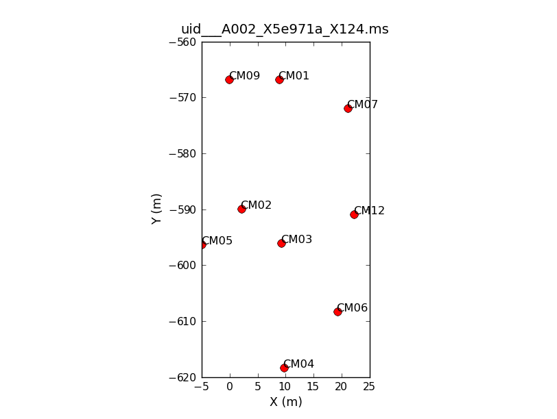
We'll now have a look at the configuration of the antennas used to take the data using the task plotants (<xr id="uid___A002_X5e971a_X124.plotants.png"/>).
<figure id="uid___A002_X5e971a_X124.plotants.png">
</figure>
# In CASA
basename=['uid___A002_X5e971a_X124','uid___A002_X5e971a_X2e7','uid___A002_X5e9ff1_X3f3','uid___A002_X5e9ff1_X5b3', 'uid___A002_X60b415_X44','uid___A002_X62f759_X4eb']

for asdm in basename:
    print "Antenna configuration for : "+asdm
    plotants(vis=asdm+'.ms', figfile=asdm+'.plotants.png')
    clearstat()
    dummy_string = raw_input("Hit <Enter> to see the antenna configuration for the next data set.")
This will loop through all 6 data sets, show you the antenna position for each, and save that as a file named, e.g., "uid___A002_X5e971a_X124.plotants.png" for the first data set. The "raw_input" command asks CASA to wait for your input before proceeding. If you would prefer to just browse the .png files after the fact you can remove this. Notice that the antenna setup changes, but only slightly, over the course of the 6 data sets.
- In CASA
basename=['uid___A002_X5e971a_X124','uid___A002_X5e971a_X2e7','uid___A002_X5e9ff1_X3f3','uid___A002_X5e9ff1_X5b3', 'uid___A002_X60b415_X44','uid___A002_X62f759_X4eb']
for asdm in basename_all:
   print "Antenna configuration for : "+asdm
   plotants(vis=asdm+'.ms', figfile=asdm+'.plotants.png')
   clearstat()
   dummy_string = raw_input("Hit <Enter> to see the antenna configuration for the next data set.")
</source>
This will loop through all 6 data sets, show you the antenna position for each, and save that as a file named, e.g., "uid___A002_X5e971a_X124.plotants.png" for the first data set. The "raw_input" command asks CASA to wait for your input before proceeding. If you would prefer to just browse the .png files after the fact you can remove this. Notice that the antenna setup changes, but only slightly, over the course of the 6 data sets.
How to Deal With 6 Measurement Sets
# In CASA
basename=['uid___A002_X5e971a_X124','uid___A002_X5e971a_X2e7','uid___A002_X5e9ff1_X3f3',
'uid___A002_X5e9ff1_X5b3', 'uid___A002_X60b415_X44','uid___A002_X62f759_X4eb']

for asdm in basename_all:
    print asdm
You only need to define your list of MS files once per CASA session. Then "basename" will be a variable in the casapy shell. You can check if it exists by typing "print basename". In the interests of allowing you to easily exit and restart CASA and pick this guide up at any point we will redefine "basename" in each section of the guide. Feel free to skip this step if you've already defined it in your session.
This page will step you through the reduction of the M100 Band3 SV data set using these 'for' loops. We will not be able to show every diagnostic plot but we give an example of each and the syntax to generate the rest. Also please be aware that even on a very fast machine this whole process can take a while, we are simply dealing with a lot of data.
A Priori Flagging
Even before we look in detail, we know that there are some data that we wish to exclude. We will start by flagging "shadowed" data where one antenna blocks the line of sight of another. We will also flag scans that were used to carry out pointing and atmospheric calibration, identified by their scan intent. Finally, we'll flag the autocorrelation data (the correlation of the signal from an antenna with itself) as we are only interested in cross-correlation data to make an interferometric image.
Start by defining our list of MS files:
# In CASA
basename=['uid___A002_X5e971a_X124','uid___A002_X5e971a_X2e7','uid___A002_X5e9ff1_X3f3','uid___A002_X5e9ff1_X5b3', 'uid___A002_X60b415_X44','uid___A002_X62f759_X4eb']
You may want to reset the flagging if you have tried this step before and are starting over though this is not necessary on your first time through. Do so using flagdata:
# In CASA
for asdm in basename:
    print "Resetting flags for "+asdm
    flagdata(vis=asdm+'.ms', mode='unflag', flagbackup=F)
Then flag shadowed data using the command flagdata:
# In CASA
for asdm in basename:
    print "Flagging shadowed data for "+asdm
    flagdata(vis=asdm+'.ms',mode = 'shadow', flagbackup = F)
In the flagdata task we choose:
- vis = asdm+'.ms' : each measurement set
- mode = 'shadow': flag shadowed data
- flagbackup = F: Do not automatically back up the flag files. We will save all of the a priori flags together using flagmanager at the end of this subsection and save some space and time.
The relevant calibration information has already been extracted from the pointing and atmospheric scans and we will not need them below. Now flag the pointing scans using flagdata in 'manualflag' mode and selecting on 'intent':
# In CASA
for asdm in basename:
    print "Flagging calibration scans for "+asdm
    flagdata(vis=asdm+'.ms', mode='manual', intent='*POINTING*,*SIDEBAND_RATIO*,*ATMOSPHERE*', flagbackup = F)
Note that because the atmospheric calibration scans contain only TDM spectral windows, they will be removed automatically when we separate out the FDM data below.
Now flag the autocorrelation data:
# In CASA
for asdm in basename:
    print "Flagging autocorrelation data for "+asdm
    flagdata(vis=asdm+'.ms',autocorr=True,flagbackup=F)
# In CASA
for asdm in basename:
    print "Flagging shadow for "+asdm
    flagmanager(vis = asdm+'.ms', mode = 'restore', versionname = 'shadow')
Finally store the current flags information using flagmanager:
# In CASA
for asdm in basename:
    print "Backing up 'a priori' flags for "+asdm
    flagmanager(vis = asdm+'.ms', mode = 'save', versionname = 'Apriori')
The flagmanager task will also allow you to view the saved flagging versions,
including those created by running flagdata with flagbackup=T.

For example try

flagmanager(vis='uid___A002_X5e971a_X124.ms', mode='list')

The output in the logger should list the Apriori flagging that we have applied.
It will also indicate versions associated with any flagdata command where you
did not set flagbackup=F. Other tasks, for example applycal, will also create
flag version tables.
Create and Apply Tsys and Antenna Position Calibration Tables
#In CASA
basename=['uid___A002_X5e971a_X124','uid___A002_X5e971a_X2e7','uid___A002_X5e9ff1_X3f3','uid___A002_X5e9ff1_X5b3', 'uid___A002_X60b415_X44','uid___A002_X62f759_X4eb']
Tsys
The Tsys calibration gives a first-order correction for the atmospheric opacity as a function of time and frequency and associates weights with each visibility that persists through imaging.
Use gencal to create the Tsys calibration tables from the spectral windows with CALIBRATE_ATMOSPHERE intents in listobs. Later in the applycal stage this TDM Tsys table will be interpolated to the FDM.
#In CASA
basename=['uid___A002_X5e971a_X124','uid___A002_X5e971a_X2e7','uid___A002_X5e9ff1_X3f3',
'uid___A002_X5e9ff1_X5b3', 'uid___A002_X60b415_X44','uid___A002_X62f759_X4eb']

for asdm in basename:
  os.system('rm -rf cal_plots/Tsys_plots/'+asdm+'.tdm.tsys*')
  tsysfields=['3c279','Titan','M100']
  caltable=asdm+'.tdm.tsys'
  for field in tsysfields:
    au.plotbandpass(caltable=caltable,yaxis='amp',field=field,xaxis='freq',
                showatm=True,overlay='time',
                figfile='cal_plots/Tsys_plots/'+caltable+'.'+field,buildpdf=False,
                interactive=False,chanrange='8~120',subplot=42)
This sequence loops over all of our files and plots Tsys as a function of time for channel 50 in spectral window 5. In the call to plotcal: The Tsys values in CM01 and CM07 are too high.
- subplot=421 parameter sets up a 4 x 2 panel grid.
- iteration tells plotcal to make a separate plot for each antenna.
- spw '5:50~50' selects spw '5' channel 50-50. This allows us to cleanly separate time variations from frequency variations.
Because 8 panels (2 panels for each antenna - LSB and USB) is not enough to show all antennas on one page, there are two plotcal calls: one for the first 8 antennas (antenna=0~7), and then for the remaining antennas (antenna=8~15). The fontsize needs to be set to a small value or the text overlaps.
The 'raw_input' commands will wait for you to hit Enter before issuing the next plot command. In the example above these are commented out (the leading "#" means that CASA will ignore them). If you would like to interactively cycle through the plots, uncomment them by removing the "#". Otherwise, the figfile parameter directs the output to .png files for later inspection. The easiest way to look at the 20 plots produced here is to simply inspect the .png files using your favorite viewer.
We will also want to look at Tsys as a function of frequency. This will use the analysisutils package mentioned at the beginning of this guide (called by the au. command)
#In CASA
basename=['uid___A002_X5e971a_X124','uid___A002_X5e971a_X2e7','uid___A002_X5e9ff1_X3f3','uid___A002_X5e9ff1_X5b3',
'uid___A002_X60b415_X44','uid___A002_X62f759_X4eb']
for name in basename:
    os.system('rm -rf name+'.ms.tsys')
    gencal(vis = name+'.ms',
       caltable=name+'.ms.tsys',
       caltype = 'tsys')
<figure id="uid___A002_X5e971a_X124.spw8.t0.png">
</figure> <figure id="uid___A002_X5e971a_X124.spw10.t3.png">
</figure>
<figure id="uid___A002_X5e971a_X124.spw14.t1.png">
</figure>
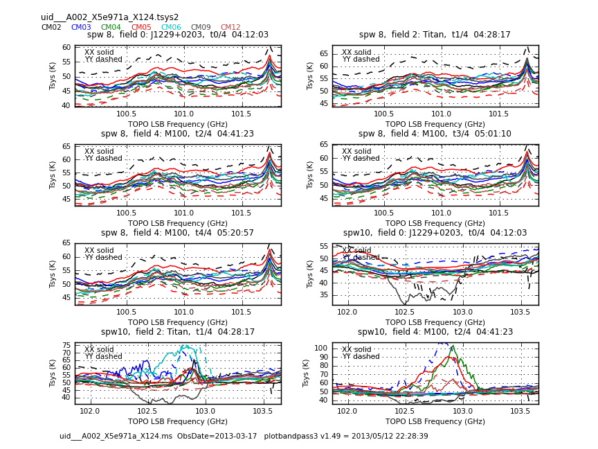
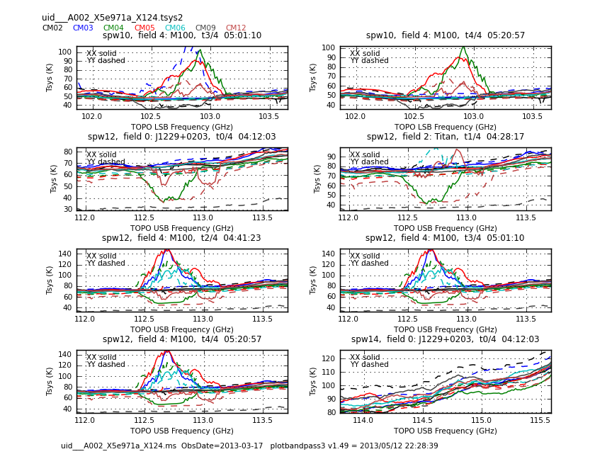
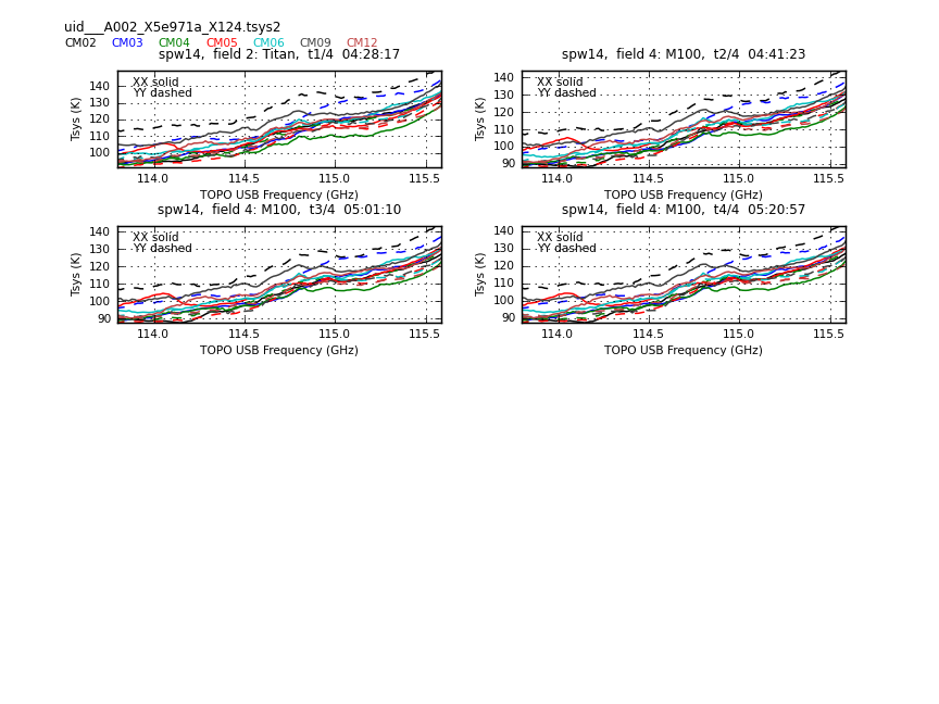
Now have a look at the Tsys vs. frequency plots or see <xr id="uid___A002_X5e971a_X124.spw8.t0.png"/>, <xr id="uid___A002_X5e971a_X124.spw10.t3.png"/>, and <xr id="uid___A002_X5e971a_X124.spw14.t1.png"/> for examples on the first data set. You can see the effect of a close pair of atmospheric ozone absorption lines at about *** GHz that makes Tsys larger near that frequency in all antennas. Applying the Tsys calibration tables will minimize the contribution of these atmospheric lines.
Antenna Positions
The antenna position table reflects refinements in the measured positions of the antennas from those stored in the data. gencal will now be used put antenna position data into each observation. Again, gencal will merely append to existing antenna position data, ruining any subsequent results. We start by removing any existing antenna position refinements, followed by defining the antenna names, then their refinements (both as arrays), finally running gencal to create the information CASA can refer to for antenna positions.
#In CASA
os.system('rm -rf name+'.ms.antpos')
gencal(vis = 'X2e7.ms',
       caltable = 'X2e7.ms.antpos',
       caltype = 'antpos',
       antenna = 'CM02,CM03,CM04,CM05,CM06,CM07,CM09,CM12',
       parameter = [-1.04341656e-04,4.29447740e-04,4.12447378e-04,1.04838982e-05,4.57765535e-04,3.53057869e-04,
1.38600077e-03,-6.59998506e-04,-4.26100381e-03, -8.91945325e-04,4.27036546e-04,1.40665658e-03,-1.16256997e-04,
2.12460477e-03,-5.08893328e-03,-3.65406508e-03,1.86459431e-02,5.67199755e-03,8.04639747e-03,4.01791865e-02,
1.46969082e-03,-5.75850718e-05,6.55882061e-04,7.88089819e-05])

#In CASA
gencal(vis = 'X3f3.ms',
       caltable = 'X3f3.ms.antpos',
       caltype = 'antpos',
       antenna = 'CM02,CM03,CM04,CM05,CM06,CM07,CM09,CM12',
       parameter = [-1.04341656e-04,4.29447740e-04,4.12447378e-04,1.04838982e-05,4.57765535e-04,3.53057869e-04,
1.38600077e-03,-6.59998506e-04,-4.26100381e-03,-8.91945325e-04,  4.27036546e-04,1.40665658e-03,-1.16256997e-04,
2.12460477e-03,-5.08893328e-03,-3.65406508e-03,1.86459431e-02,5.67199755e-03,8.04639747e-03,4.01791865e-02,
1.46969082e-03,-5.75850718e-05,6.55882061e-04,7.88089819e-05])


#In CASA
gencal(vis = 'X5b3.ms',
       caltable = 'X5b3.ms.antpos',
       caltype = 'antpos',
       antenna = 'CM02,CM03,CM04,CM05,CM06,CM09,CM12',
       parameter = [-1.04341656e-04,4.29447740e-04,4.12447378e-04,1.04838982e-05,4.57765535e-04,3.53057869e-04,
1.38600077e-03,-6.59998506e-04,-4.26100381e-03,-8.91945325e-04,4.27036546e-04,1.40665658e-03,-1.16256997e-04,
2.12460477e-03,-5.08893328e-03,8.04639747e-03,4.01791865e-02,1.46969082e-03,-5.75850718e-05,6.55882061e-04,7.88089819e-05])


#In CASA
gencal(vis = 'X44.ms',
       caltable = 'X44.ms.antpos',
       caltype = 'antpos',
       antenna = 'CM12,CM02,CM03,CM05',
       parameter = [5.70082944295e-05,-0.00065711393962,-7.91980095891e-05,0.000104837426825,-0.000430660050663,
-0.000411915081903,-1.1060689293e-05,-0.000458996548728,-0.00035344706733,
                    0.000982235185802,-0.000412690453231,-0.00145998690277])
gencal(vis = 'X44.ms',
       caltable = 'X44.ms.antpos',
       caltype = 'antpos',
       antenna = 'CM02',
       parameter = [0.0,0.0,0.0])


#In CASA
gencal(vis = 'X124.ms',
       caltable = 'X124.ms.antpos',
       caltype = 'antpos',
       antenna = 'CM02,CM03,CM04,CM05,CM06,CM07,CM09,CM12',
       parameter = [-1.04341656e-04,4.29447740e-04,4.12447378e-04,1.04838982e-05,4.57765535e-04,3.53057869e-04,
1.38600077e-03,-6.59998506e-04,-4.26100381e-03,-8.91945325e-04,4.27036546e-04,1.40665658e-03,-1.16256997e-04,
2.12460477e-03,-5.08893328e-03,-3.65406508e-03,1.86459431e-02,5.67199755e-03,8.04639747e-03,4.01791865e-02,
1.46969082e-03,-5.75850718e-05,6.55882061e-04,   7.88089819e-05])
gencal(vis = 'X124.ms',
       caltable = 'X124.ms.antpos',
       caltype = 'antpos',
       antenna = 'CM02',
       parameter = [0.0,0.0,0.0])
Applycal
We are now ready to apply the Tsys tables to the data with applycal, which reads the specified gain calibration tables, applies them to the (raw) data column, and writes the calibrated results into the corrected column. Again, we loop through all the datasets. It is important to only apply Tsys and WVR corrections obtained close in time to the data being corrected, so in addition to looping over data sets we define the list of unique source names and loop over these. Then by setting gainfield and field to the same value we ensure that Tsys and WVR calibrations are only applied to the source for which they are measured. Because the source has a different name in the Northern Mosaic and the Southern Mosaic, we will carry out two loops. We will only correct spw 1 and 3, our science windows, because we will drop the other data in a moment.
The applycal task now has much more flexibility for interpolating and applying calibrations derived in one spectral window to another, even if they do not share the same spectral shape (number of channels and channel width). This new functionality is used below to interpolate the TDM (128 channel) Tsys measurements to the FDM (3840 channel) spectral windows. This is controlled through the spectral window mapping parameter *spwmap*. Because this can be a bit confusing, we've written a "helper" function that will tell you what you should put for the Tsys calibration table part of spwmap. We only need to run it on one of the datasets because they are all the same in this regard
# In CASA
from recipes.almahelpers import tsysspwmap
tsysspwmap(vis='uid___A002_X207fe4_X3a.ms',tsystable='uid___A002_X207fe4_X3a.tdm.tsys')
This will print to your screen: [0, 5, 5, 7, 5, 5, 5, 7]. Recall that the TDM spectral windows are spw=5 and 7 and the FDM spectral windows are 1 and 3. This spwmap tells applycal to use the Tsys information in spectral window 5 for spectral window 1; and to use the information in spectral window 7 for spectral window 3. Beyond that, it is only important that there are placeholders for the other spectral windows, its also useful to note that you need not give placeholders for spectral window ids larger than the largest spectral window you need to use, in this case 7.
You will also need to put in placeholders for other tables that you give the gaintables. So if the Tsys table is 2nd in the list, spwmap=[[],[0,5,5,7,5,5,5,7],[]]
Now run the applycal commands.
# In CASA

# A new list of file names that contain only data from the Northern Mosaic
basename=['uid___A002_X5e971a_X124','uid___A002_X5e971a_X2e7','uid___A002_X5e9ff1_X3f3',
'uid___A002_X5e9ff1_X5b3', 'uid___A002_X60b415_X44','uid___A002_X62f759_X4eb']
field_names = ['Titan','3c279','NGC*']

for asdm in basename_north:
    print "Apply Tsys and Antenna Position calibrations to "+asdm
    for field in field_names:
        applycal(vis=asdm+".ms", spw='1,3',
            field=field, gainfield=['',field,field],
            interp=['','linear,spline','nearest'],
            gaintable=[asdm+'.antpos',asdm+'.tdm.tsys'],
            spwmap=[[],[0, 5, 5, 7, 5, 5, 5, 7],[]],
            flagbackup=F, calwt=T)
where:
- field: the field to which we will apply the calibration,
- gainfield: the field from which we wish to take the calibration table
- interp = 'nearest' : apply the nearest solution from the calibration table rather than interpolating.
As you browse through the whole data set, you will probably note some problems along the same lines as the DV04 issue we saw above. We'll apply these as additional data flagging in just a moment.
Inspect Data
We are not quite done with the original ".ms" data sets yet. Before going further it will be useful to use plotms to show the effects of applying the calibration. In the process we'll take a quick look at each antenna and search for pathologies in the data.
For this basic inspection, we want to compare the phase and amplitude as a function of frequency and time in the DATA and CORRECTED columns of each measurement set. The CORRECTED column has had the Tsys and WVR calibrations applied and so we expect lower phase scatter and flatter amplitude response as a function of time and frequency. We are looking for antenna-based issues, so cycling through a set of baselines that includes each antenna once will be a good start. We'll focus these plots on the phase+bandpass calibrator, 3c279, and on baselines that include antenna CM04, which we will make our reference antenna in just a bit.
Each CASA Measurement Set has up to three "columns" of data: DATA, CORRECTED, and MODEL (though it is possible
for a MS to hold only a DATA column if it has not been processed at all).

A column entry exists for each data point (baseline, frequency, time).

The DATA column holds the current raw data, though using split as we just did we can change the definition of
"raw" data.

The CORRECTED column holds the result of applying one or more calibration tables (e.g., via applycal) to the
DATA column and so represents a corrected version of the DATA column.

In CASA 4.1: the MODEL column is deprecated (though it is still possible to use them by explicitly setting usescratch=T).
Instead, the model is stored in the header of the ms. This is a great step forward in terms of saving space and time
to create scratch columns

To get an intuitive feel for the columns you may wish to explore using plotms (which can plot different data
columns, as seen below) or the browsetable task.
<figure id="plotms_amp_vs_freq_example-data.png">
</figure> <figure id="plotms_amp_vs_freq_example-corr.png">
</figure>
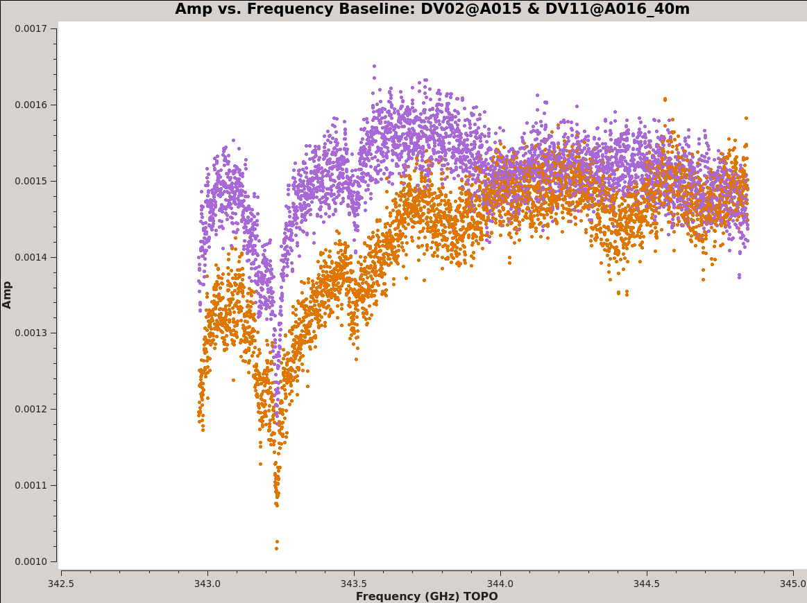
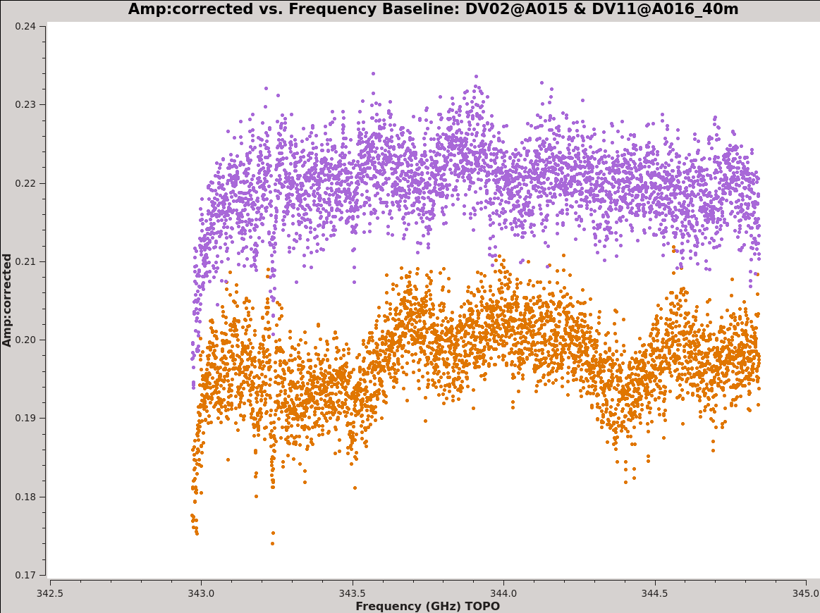
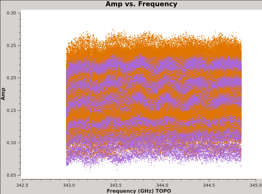
First, we plot amplitude as a function of frequency for 3c279. We start by plotting the DATA column, set color to indicate the two correlations (i.e., the XX and YY polarizations), and ask plotms to iterate over baseline. By setting antenna to 'DV11&*' we select only baselines that include DV11. We ask plotms to average all data over a very long timescale, avgtime = 1e8 seconds ~ 3 years or much longer than the time spanned by the whole data set. By setting avgscan = True we allow plotms to average across scan boundaries. The result is a plot of average amplitude per channel vs. frequency.
# In CASA
basename_all=["uid___A002_X1ff7b0_Xb","uid___A002_X207fe4_X3a","uid___A002_X207fe4_X3b9",
     "uid___A002_X2181fb_X49","uid___A002_X1ff7b0_X1c8","uid___A002_X207fe4_X1f7",
     "uid___A002_X207fe4_X4d7","uid___A002_X215db8_X18","uid___A002_X215db8_X1d5",
     "uid___A002_X215db8_X392"]

asdm=basename_all[0]

plotms(vis=asdm+'.ms',
       field='3c279',
       xaxis='frequency', yaxis='amp',
       selectdata=T, spw='1',
       avgtime='1e8',avgscan=T,
       coloraxis='corr',
       iteraxis='baseline',
       antenna='CM04&*',
       ydatacolumn='data')
Notice the green arrows along the bottom of the plotms window. We asked plotms to iterate over baseline. As you click the arrows, the plot will rotate from baseline to baseline, always with DV11 so that each antenna shows up once. To see the effect of the calibration, go to the "Axes" tab along the left of the plotms window and pull down the Data Column menu under the Y Axis. Set this from DATA to CORRECTED and you should see the effects of the calibration. You may need to ensure that the "Force Reload" box is checked before clicking "Plot" (both buttons lie at the bottom of the panel). For the most part things get better (flatter), but as we noted before DV04 is problematic.
<figure id="plotms_amp_vs_time_north.png">
</figure> <figure id="plotms_amp_vs_time_south.png">
</figure>
You can now make analogous calls to examine the phase vs. frequency, amplitude vs. time, and phase vs. time.
# In CASA
plotms(vis=asdm+'.ms',
       field='3c279',
       xaxis='frequency', yaxis='phase',
       selectdata=T, spw='1',
       avgtime='1e8',avgscan=T,
       coloraxis='corr',
       iteraxis='baseline',
       antenna='CM04&*',
       ydatacolumn='data')

plotms(vis=asdm+'.ms',
       field='3c279',
       xaxis='time', yaxis='amp',
       selectdata=T, spw='1:1200~1300',
       avgchannel='1000',avgscan=F,
       coloraxis='corr',
       iteraxis='baseline',
       antenna='CM04&*',
       ydatacolumn='data')

plotms(vis=asdm+'.ms',
       field='3c279',
       xaxis='time', yaxis='phase',
       selectdata=T, spw='1:1200~1300',
       avgchannel='1000',avgscan=F,
       coloraxis='corr',
       iteraxis='baseline',
       antenna='CM04&*',
       ydatacolumn='data')
Where:
- spw is set to cover only channels 1200~1300 for the time plots in order to isolate time dependent variations from frequency-dependent behavior. Those 101 channels represent only a small part of the total spw 1 bandpass.
- avgchannel set to a large number causes the plots of phase and amplitude vs. time to average data at all frequencies into a single point for each measurement.
- coloraxis corr sets the colors to correspond to the two polarizations of the data.
In each case, you will want to examine each baseline, alternating between the DATA and CORRECTED columns.
This is a lot of data inspection and that's only for one of 10 data sets! You can iterate across the data by hand, updating "asdm" to refer to each data set in order and cycling between baselines and DATA/CORRECTED. It is also possible to script CASA to show you the key plots in succession (see the next block down). However you approach the infrastructure, you are looking for:
- Improved scatter and lower variability in phase and amplitude vs. frequency and time. This indicates that the WVR and Tsys calibrations helped.
- Sudden jumps in phase or amplitude as a function of either time or frequency. These may indicate problems with the antenna during that observation.
- Large gradients, especially full wraps, in phase as a function of frequency. This may indicate a problem in the delays, the signal path length to the telescopes.
- Unusual magnitude, scatter, or patterns in any plot - though this may be better explored using plots that show all data together, which we'll make in a moment.
- Missing data. For example, if the phase calibrator drops out for a period of time we will not be able to calibrate and will need to flag the data.
As you look through, note individual potentially problematic antennas. If all antennas in a data set appear problematic it may be that your "reference" antenna, DV11 in the example above, is the source of the problem. In this case swap this reference antenna for another and see whether the problem is isolated to your original reference antenna.
A brief aside on structure:

This section (Data Inspection) and the next (Apply Flags) are closely linked. We will present them as two
separate steps. The idea here is that you look through your data, note problems, and then write commands to
flag problematic data. This mimics one approach to writing data reduction scripts for CASA, where you will
group all flagging together into one convenient place. Other CASA guides take a different approach, interleaving
flagging and plotting. There is no "right" answer here. Find an approach to data inspection that works for you.
If you do wish to semi-automate the plot generation, the following sequence will cycle between data and corrected plots for each data set in turn. Type "stop" at any input call to break out.
Note: In loops like this involving plotms, hitting enter before the last dataset completes loading may cause plotms to stop refreshing the plot window at each step, or cause the window to disappear altogether. This will be fixed in an upcoming CASA release. Right now, you may need to exit CASA and restart to bring up the plotms window again, but you should be able to continue in the script where you left off.
# In CASA

user_input = ""
for asdm in basename_all:
    # check if a stop has been requested
    if user_input == "stop":
        break
    # Extract antenna list for this data set.
    tb.open(asdm+'.ms/ANTENNA', nomodify=True)
    ants = tb.getcol('NAME')
    tb.close
    # Define the reference antenna to make baselines with
    ref_ant = 'DV11'
    # Loop over antennas
    for ant in ants:
        # Check if the user wants to stop
        if user_input == "stop":
            break
        # Skip correlation of reference antenna with itself (autocorrelations are flagged anyhow)
        if ant == ref_ant:
            continue
        # Define the baseline with the reference antenna for current antenna
        ant_str = ref_ant+'&'+ant
        print "Showing baseline "+ant_str+" for data set "+asdm
        print "Use this to inspect effect of applying wvrcal and Tsys calibrations."
        # Loop over phase and amplitude as axes
        for y_axis in ["amp", "phase"]:
            # Make 'before' plot for frequency x-axis
            print "... "+y_axis+" vs. frequency for DATA:"
            plotms(vis=asdm+'.ms', spw='1', field='3c279',
               antenna=ant_str, xaxis="frequency", yaxis=y_axis,
               avgtime="1e8", avgscan=T, coloraxis="corr",
               ydatacolumn="data")
            user_input = raw_input("Hit <ENTER> to see CORRECTED data [type 'stop'+<Enter> to break out].")
            if user_input == "stop":
                break
            # Make 'after' plot for frequency x-axis
            print "... "+y_axis+" vs. frequency for CORRECTED:"
            plotms(vis=asdm+'.ms', spw='1', field='3c279',
               antenna=ant_str, xaxis="frequency", yaxis=y_axis,
               avgtime="1e8", avgscan=T, coloraxis="corr",
               ydatacolumn="corrected")
            user_input = raw_input("Hit <ENTER> to proceed to next plot [type 'stop'+<Enter> to break out].")
            if user_input == "stop":
                break
            # Make 'before' plot for time x-axis
            print "... "+y_axis+" vs. time for DATA:"
            plotms(vis=asdm+'.ms', spw='1:1200~1300', field='3c279',
               antenna=ant_str, xaxis="time", yaxis=y_axis,
               avgchannel="1000", coloraxis="corr",
               ydatacolumn="data")
            user_input = raw_input("Hit <ENTER> to see CORRECTED data [type 'stop'+<Enter> to break out].")
            if user_input == "stop":
                break
            # Make 'after' plot for time y-axis
            print "... "+y_axis+" vs. time for CORRECTED:"
            plotms(vis=asdm+'.ms', spw='1:1200~1300', field='3c279',
               antenna=ant_str, xaxis="time", yaxis=y_axis,
               avgchannel="1000", coloraxis="corr",
               ydatacolumn="corrected")
            user_input = raw_input("Hit <ENTER> to proceed to next plot [type 'stop'+<Enter> to break out].")
            if user_input == "stop":
                break
<figure id="plotms_amp_vs_uvdist_north.png">
</figure>
<figure id="plotms_amp_vs_freq_3c279.png">
</figure> <figure id="plotms_amp_vs_freq_Titan.png">
</figure> <figure id="plotms_amp_vs_freq_Antennae.png">
</figure>
A detailed explanation of the procedure is a bit outside the scope of this guide (for more on python see http://www.python.org/ and for more on the CASA toolkit see http://casa.nrao.edu/), but the basic process is to loop over each data set, baseline with the reference antenna (here DV11), and y-axis of interest (phase or amplitude) then plot the effect of the calibration vs. frequency and time for each combination. Running this to step through the data will give you about 200 "before and after" plots from which you could note a subset of problematic cases to be followed up by hand. Many other strategies to inspect the data are also viable.
With the Tsys and WVR calibrations applied successfully and the a priori flagging taken care of we will now split out the corrected data. We will keep only the corrected data, specified via datacolumn, and only spectral window 1, which contains the FDM (high spectral resolution) observations of the CO(3-2) line. Setting keepflags=F tells split not to carry over any fully flagged rows from the original data set to the new MS. We give the new MS files the extension ".wvrtsys.ms" to indicate that they have been corrected for WVR and Tsys effects. Because split will not overwrite existing files, we remove any previous versions of the new MS before beginning.
# In CASA
for asdm in basename_all:
    os.system('rm -rf '+asdm+'.wvrtsys.ms')
    print "Splitting out corrected data for "+asdm
    split(vis=asdm+'.ms', outputvis=asdm+'.wvrtsys.ms',
        datacolumn='corrected', spw='1', keepflags=F)
Be patient, split may take awhile. The WVR and Tsys-corrected data now sit in the DATA column of the new measurement sets, which have only one spectral window (now labeled spectral window 0 though it was spectral window 1 in the original data). You may wish to run listobs to illustrate the changes:
# In CASA
for asdm in basename_all:
    os.system('rm '+asdm+'.wvrtsys.listobs.txt')
    listobs(vis=asdm+'.wvrtsys.ms', listfile=asdm+'.wvrtsys.listobs.txt', verbose=True)
Note the new spectral window information:
2011-08-05 01:07:08 INFO listobs	Spectral Windows:  (1 unique spectral windows and 1 unique polarization setups)
2011-08-05 01:07:08 INFO listobs	  SpwID  #Chans Frame Ch1(MHz)    ChanWid(kHz)TotBW(kHz)  Ref(MHz)    Corrs
2011-08-05 01:07:08 INFO listobs	  0        3840 TOPO  344845.586  488.28125   1875000     344908.33   XX  YY
Next we will do a bit more inspection using plotms to look at whole data sets. This will help us identify missing data or look for egregious outliers.
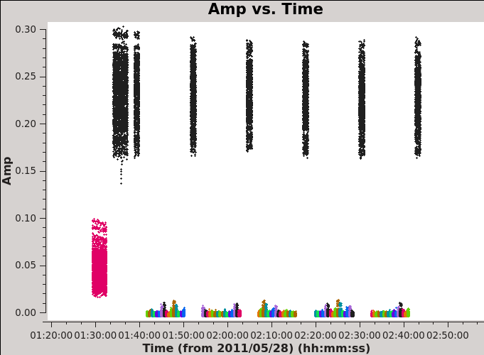
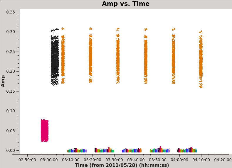
First we plot amplitude versus time (see <xr id="plotms_amp_vs_time_north.png"/> and <xr id="plotms_amp_vs_time_south.png"/>), averaging over all channels (by setting avgchannel to the very large value 10,000). We colorize by field so that scans on Titan are red, the bandpass and phase calibrator 3c279 is black (and orange in the Southern Mosaic where it has two field IDs), and the Antennae mosaic appears as a range of colors (one per pointing).
# In CASA
basename=['uid___A002_X5e971a_X124','uid___A002_X5e971a_X2e7','uid___A002_X5e9ff1_X3f3','uid___A002_X5e9ff1_X5b3',
'uid___A002_X60b415_X44','uid___A002_X62f759_X4eb']

for asdm in basename_all:
    plotms(vis=asdm+'.wvrtsys.ms',
            xaxis='time', yaxis='amp',
            avgchannel='3840',coloraxis='field')
    dummy_string = raw_input("Examining amplitude vs. time for "+asdm+" . Hit <Enter> to proceed.")
Here look for:
- Missing data. The source needs to be flanked by phase calibrator scans, if those are missing for any reason we need to flag the appropriate time range.
- Dramatic outliers. Does the source suddenly get very bright or the otherwise bright calibrator appear anomalously faint for a brief time? This likely indicates problematic data that should be identified and flagged. You can use the "select" (box with green plus along the bottom row in plotms) and "locate" (magnifying glass) buttons in plotms to isolate and identify problem data (it will print to the log).
- Smooth variation with time. A sudden jump may indicate a problem and often the safest approach is to flag data near a discontinuity.
Look through the amplitudes vs. time for each data set (remember that we've already examined the phases vs. time and amplitude vs. time for individual baselines above).
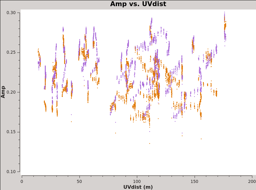
There are two other very useful "averaging" plots worth making. First, we plot amplitude as a function of u-v distance (projected antenna separation). Discontinuities and spikes in this plot are often from non-astrophysical sources. In the phase analog to the plot, the effects of atmospheric decorrelation can be assessed from increased scatter at longer u-v distances. While using the moon Titan as our flux calibrator, we may want to watch for flaring amplitudes at short u-v distances. These may indicate that Saturn is contaminating our beam. For a perfect, bright point source, we expect flat amplitudes as a function of u-v distance at the source amplitudes. <xr id="plotms_amp_vs_uvdist_north.png"/> shows an example of this plot, generated via:
# In CASA
basename=['uid___A002_X5e971a_X124','uid___A002_X5e971a_X2e7','uid___A002_X5e9ff1_X3f3','uid___A002_X5e9ff1_X5b3',
'uid___A002_X60b415_X44','uid___A002_X62f759_X4eb']

for asdm in basename_all:
    plotms(vis=asdm+'.wvrtsys.ms',
        field='3c279',
        xaxis='uvdist', yaxis='amp',
        avgchannel='4096',coloraxis='corr')
    dummy_string = raw_input("Examining amplitude vs. UV Distance for 3c279 for "+asdm+" . Hit <Enter> to proceed.")
    plotms(vis=asdm+'.wvrtsys.ms',
        field='Titan',
        xaxis='uvdist', yaxis='amp',
        avgchannel='4096',coloraxis='corr')
    dummy_string = raw_input("Examining amplitude vs. UV Distance for Titan for "+asdm+" . Hit <Enter> to proceed [type 'stop'+<Enter> to break out].")
    # check if a stop has been requested
    if dummy_string == "stop":
        break
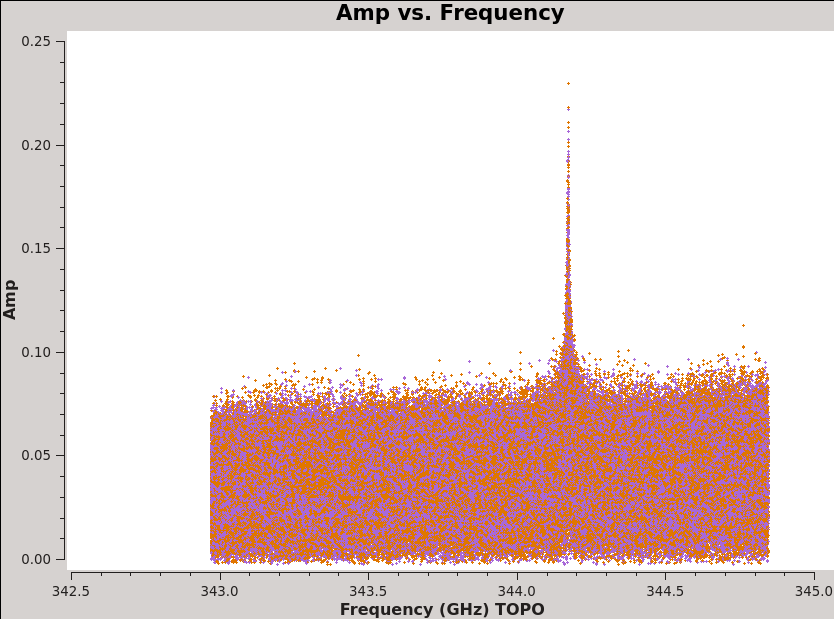
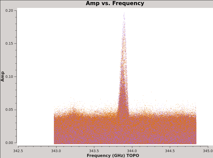
For this command notice that we can see the CO(3-2) line in the Antennae even before calibration (see <xr id="plotms_amp_vs_freq_Antennae.png"/>) and that Titan also shows evidence of a strong line (also <xr id="plotms_amp_vs_freq_Titan.png"/>)! This will need to be flagged before we can use Titan to calibrate the flux scale of our data.
This suite of plots (along with the earlier inspection of the Tsys tables) gives us the tools we need to identify problematic data through the data sets. We use this to generate a set of inspection-driven flagdata commands for each data set. We apply these before the bandpass and gain calibration.
Apply Flagging
Based on this inspection and the other plots we have made, we now flag problematic portions of the data. We break up the flags by reason for flagging in order to illustrate the process. As you reduce your own data it may be more efficient to group flags by data set and make use of the flagcmd command. Except for the "post-calibration" flagging, the inspection plots that we just looked through have already revealed all of the problems that we flag. We structure the guide so that the flagging is grouped in one place.
As before, we may wish to reset our flags before beginning (particularly if one iterates this process) via:
# In CASA

basename=['uid___A002_X5e971a_X124','uid___A002_X5e971a_X2e7','uid___A002_X5e9ff1_X3f3','uid___A002_X5e9ff1_X5b3',
'uid___A002_X60b415_X44','uid___A002_X62f759_X4eb']
for asdm in basename_all:
    flagdata(vis = asdm+'.wvrtsys.ms',mode='unflag', flagbackup = F)
Remember that we dropped the flagged data when splitting out after the WVR and Tsys calibration, so this should not undo your "A Priori" flagging of shadowed data, autocorrelations, etc.. In any case this unflagging step is not necessary during the first iteration.
- Edge Channels
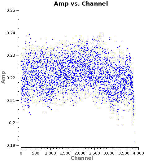
ALMA's sensitivity decreases near the edge of the baseband and it is often useful to check for a 'roll-off' in sensitivity near the edge of the band. This will appear as a downturn in amplitude as a function of channel near the edge of the window in the uncalibrated data, as a flaring due to increased noise at the spw edges in the calibrated data. It will also be visible in the amplitude part of the bandpass calibration table. Because our FDM spw does not cover the full baseband, we do not see a strong roll off in our data (see <xr id="amp_vs_channel_example.png"/>), where there is only a mild hint of a roll-off at the high end) but we do flag a (very) few channels at the high and low-frequency edge of the data set to be safe.
<figure id="amp_vs_channel_example.png">
</figure>
# In CASA

for asdm in basename_all:
    flagdata(vis = asdm+'.wvrtsys.ms', mode='manual', spw = '0:0~7,0:3831~3839', flagbackup = F)

for asdm in basename_all:
    flagdata(vis = asdm+'.wvrtsys.ms', mode='manual', spw = '0:3260~3320', flagbackup = F)
- Problematic Tsys measurements
Above we noted issues with the Tsys measurements for both DV04 and DV12. We flag the affected data. Each of these issues should be visible in the Tsys plots you made above (e.g., see <xr id="Uid___A002_X1ff7b0_Xb.tdm.tsys.3c279.DV02.spw5.CASA3_4.png"/> and <xr id="Uid___A002_X1ff7b0_Xb.tdm.tsys.3c279.PM01.spw5.CASA3_4.png"/>).
# In CASA

asdm="uid___A002_X1ff7b0_Xb"
flagdata(vis=asdm+'.wvrtsys.ms', mode='manual', antenna='DV04', flagbackup=F)

asdm="uid___A002_X207fe4_X3a"
flagdata(vis=asdm+'.wvrtsys.ms', mode='manual', antenna='DV12',correlation='YY', flagbackup=F)

asdm="uid___A002_X207fe4_X3b9"
flagdata(vis=asdm+'.wvrtsys.ms', mode='manual', antenna='DV12',correlation='YY', flagbackup=F)

asdm="uid___A002_X2181fb_X49"
flagdata(vis=asdm+'.wvrtsys.ms', mode='manual', antenna='DV12',correlation='YY', flagbackup=F)

asdm="uid___A002_X1ff7b0_X1c8"
flagdata(vis=asdm+'.wvrtsys.ms', mode='manual', antenna='DV04',flagbackup=F)

asdm="uid___A002_X207fe4_X1f7"
flagdata(vis=asdm+'.wvrtsys.ms', mode='manual', antenna='DV12',correlation='YY', flagbackup=F)

asdm="uid___A002_X207fe4_X4d7"
flagdata(vis=asdm+'.wvrtsys.ms', mode='manual', antenna='DV12',correlation='YY', flagbackup=F)

asdm="uid___A002_X215db8_X18"
flagdata(vis=asdm+'.wvrtsys.ms', mode='manual', antenna='DV12',correlation='YY', flagbackup=F)

asdm="uid___A002_X215db8_X1d5"
flagdata(vis=asdm+'.wvrtsys.ms', mode='manual', antenna='DV12',correlation='YY', flagbackup=F)

asdm="uid___A002_X215db8_X392"
flagdata(vis=asdm+'.wvrtsys.ms', mode='manual', antenna='DV12',correlation='YY', flagbackup=F)
- Unreliable Short-Spacing Measurements on Titan
<figure id="amp_vs_uv_titan_obs.png">
</figure>
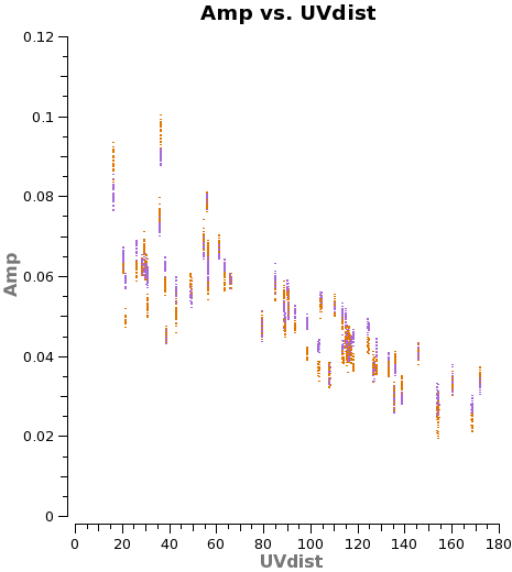
Saturn may contaminate the short u-v spacings from Titan. In any case these often show significant scatter (<xr id="amp_vs_uv_titan_obs.png"/>), so we flag them. There are still enough baselines to determine a good amplitude calibration for each antenna.
# In CASA

asdm="uid___A002_X1ff7b0_Xb"
flagdata(vis=asdm+'.wvrtsys.ms', mode='manual', field='Titan', uvrange='0~50', flagbackup = F)

asdm="uid___A002_X207fe4_X3a"
flagdata(vis=asdm+'.wvrtsys.ms', mode='manual', field='Titan', uvrange='0~40', flagbackup = F)

asdm="uid___A002_X207fe4_X3b9"
flagdata(vis=asdm+'.wvrtsys.ms', mode='manual', field='Titan', uvrange='0~50', flagbackup = F)

asdm="uid___A002_X2181fb_X49"
flagdata(vis=asdm+'.wvrtsys.ms', mode='manual', field='Titan', uvrange='0~30', flagbackup = F)

asdm="uid___A002_X1ff7b0_X1c8"
flagdata(vis=asdm+'.wvrtsys.ms', mode='manual', field='Titan', uvrange='0~50', flagbackup = F)

asdm="uid___A002_X207fe4_X1f7"
flagdata(vis=asdm+'.wvrtsys.ms', mode='manual', field='Titan', uvrange='0~30', flagbackup = F)

asdm="uid___A002_X207fe4_X4d7"
flagdata(vis=asdm+'.wvrtsys.ms', mode='manual', field='Titan', uvrange='0~30', flagbackup = F)
- Delay Issues
<figure id="phase_vs_freq_DV13.png">
</figure>
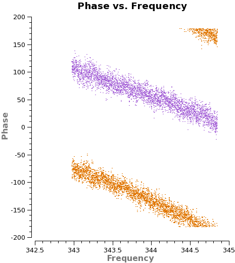
DV13 and a few other antennas show signatures of an imperfect delay calibration. This is most easily identified via strong "wrapping" of phase as a function of frequency (see <xr id="phase_vs_freq_DV13.png"/>). Such effects can be calibrated out with mild delay issues largely accounted for by the bandpass solution. The phase wrapping in DV13 seems weak enough that we will trust the calibrations to remove it. For a more extreme example see the CASA guide describing the calibration of NGC3256Band3.
- Missing Phase Calibrator Observations
<figure id="amp_vs_time_missing_scans.png">
</figure>
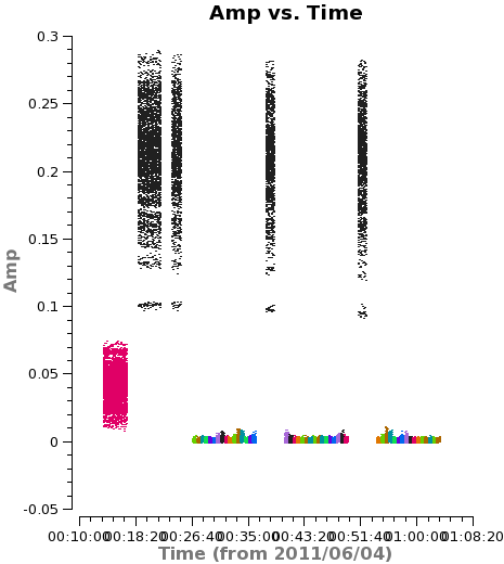
As a general rule, we want to be sure that observations of the phase calibrator (3c279) bracket each source observation. Two of the data sets do not include a final phase calibrator observation (see <xr id="amp_vs_time_missing_scans.png"/>) and for those two cases we flag the affected source observations.
# In CASA

asdm="uid___A002_X207fe4_X3b9"
flagdata(vis=asdm+'.wvrtsys.ms', mode='manual', timerange='00:53:47~01:08:00',flagbackup = F)

asdm="uid___A002_X215db8_X18"
flagdata(vis=asdm+'.wvrtsys.ms', mode='manual', antenna='DV10',timerange='19:46:20~20:34:40',flagbackup=F)
- Unexpected Scatter or Discontinuity in the Data
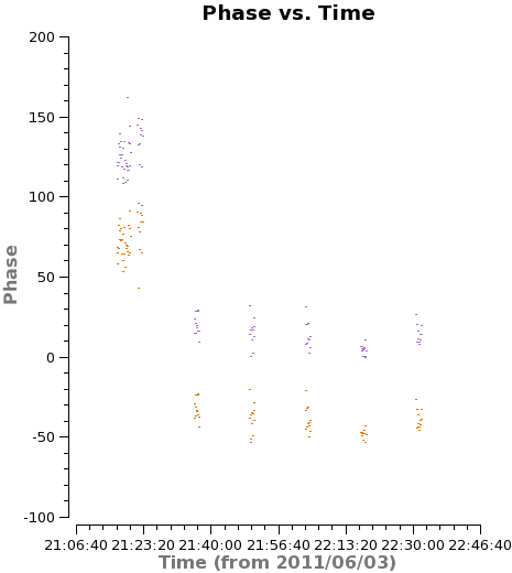
For several antennas we find sudden jumps in the phase of the phase calibrator as a function of time. These are visible in the plots of uncalibrated phase vs. time for single baselines above, and we show an example in <xr id="phase_vs_time_DV09.png"/>. It will not be possible to effectively interpolate the phase between measurements when we see these discontinuities. The safest approach is to flag the source data across these jumps. We do so here (though note that the last two flaggings are borderline cases).
<figure id="phase_vs_time_DV09.png">
</figure>
# In CASA

asdm="uid___A002_X207fe4_X3a"
flagdata(vis=asdm+'.wvrtsys.ms', mode='manual', antenna='DV09', timerange='21:24:09~21:35:35', flagbackup = F)

asdm="uid___A002_X207fe4_X1f7"
flagdata(vis=asdm+'.wvrtsys.ms', mode='manual', antenna='DV09',timerange='23:30:52~24:10:00',flagbackup=F)
flagdata(vis=asdm+'.wvrtsys.ms', mode='manual', antenna='PM01',timerange='23:16:50~24:10:00',flagbackup=F)
flagdata(vis=asdm+'.wvrtsys.ms', mode='manual', antenna='PM03',timerange='23:16:50~24:10:00',flagbackup=F)
- Outliers Visible After Calibration
<figure id="amp_vs_uvdist_outliers.png">
</figure>
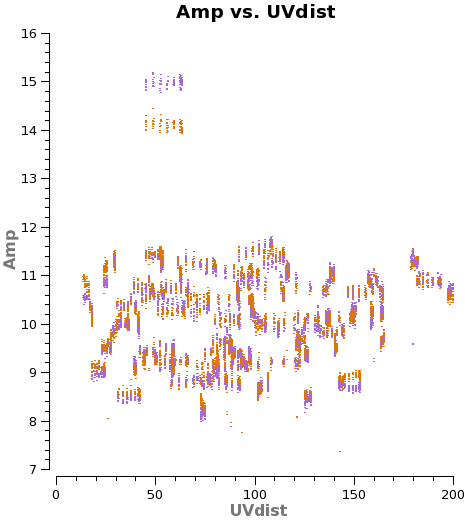
Often issues with the data may become evident after calibration (i.e., after the next few steps that we apply). These data can appear as outliers in diagnostic plots for the calibrated data or even show up in the imaging stages. Once these are identified, best practice is to apply this new flagging then redo the calibration (if the issue is very minor, then re-calibrating may not be necessary).
# In CASA
asdm="uid___A002_X207fe4_X3a"
flagdata(vis=asdm+'.wvrtsys.ms', mode='manual', timerange='21:18:00~21:22:15', flagbackup=F)

asdm="uid___A002_X2181fb_X49"
flagdata(vis=asdm+'.wvrtsys.ms', mode='manual', antenna='DV01&DV04', flagbackup=F)
Now that we've applied our flagging, back up the flags as version "User" using flagmanager:
# In CASA
basename=['uid___A002_X5e971a_X124','uid___A002_X5e971a_X2e7','uid___A002_X5e9ff1_X3f3','uid___A002_X5e9ff1_X5b3',
'uid___A002_X60b415_X44','uid___A002_X62f759_X4eb']

for asdm in basename_all:
    flagmanager(vis=asdm+'.wvrtsys.ms',mode='save',versionname ='User')
Applying this flagging will remove the most egregious pathologies from the data. We are now ready to calibrate the