N891 simdata (CASA 3.4)
↵ Simulating Observations in CASA
- This is an advanced simulation tutorial. New users are recommended to begin with the Simulation Guide for New Users (CASA 3.4).
- This guide is applicable to CASA version 3.4. For older versions of CASA see N891 simdata2.
- To create a script of the Python code on this page see Extracting scripts from these tutorials.
This tutorial simulates ALMA interferometric data for a nearby edge-on spiral galaxy.
Roughly modeled after NGC891
Data
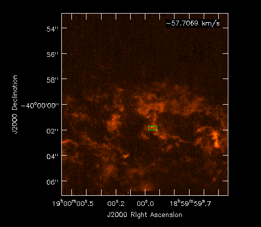
For our model, we will use a data cube of 13CO from the Galactic Ring Survey on the 14-meter FCRAO. To speed the simulation, this FITS file contains the data we want binned to a coarser velocity resolution.
Simulation
To begin, reset all simobserve parameters to their default values, set project to define the prefix for all output files, and set skymodel to the above FITS file.
# In CASA
# Initializing simobserve
# Laying down some basic ground rules
default 'simobserve'
project = 'n891d'
skymodel = 'grs-12kms.fits'
The FITS image uses units of Kelvin for brightness. simobserve expects the brightness to be specified in units of Janskys per pixel. We can convert to Janskys per steradian using the Rayleigh-Jeans law: Jy/Sr = 2x10²³ k T / λ2 = 4x10⁸T at 110GHz.
# In CASA
# Setting the new frequency of the central channel
incenter = '110.1777GHz'
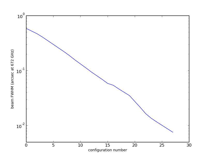
We want to simulate an observation of this model data as though it were 10-Mpc distant. The Galactic Ring Survey resolution is 40" at ~10 kpc, which translates to 0.04" at 10 Mpc. The plot at right shows how the synthesized beam size changes with the full science array configurations provided with CASA. For a 100-GHz observation, configuration 20 will give us the appropriate synthesized beam size.
If we intend to set incell=0.2arcsec in simobserve, then the cube needs to be multiplied by 4x108 * (.04/206265)2 = 1.4x10⁻⁵ to obtain Jy/pixel. The cube peaks at ~20K, so we can perform the simulation with inbright=3e-4, which should yield a peak of ~1mJy/bm.
- Will we be dominated by the noise in the input model? Input noise ~150mK or S/N~20, so at our scaled intensity, ~0.05 mJy/bm. The ALMA Sensitivity Calculator says that ALMA will achieve 2.5mJy/bm in 2 hours for the input 212m/s channel width (0.075MHz), so the noise in the input model should not affect our results.
# In CASA
# Setting the new channel width
inwidth = '0.075MHz'
- We do have a sensitivity issue though - if we decrease the spectral resolution by a factor of 6 (bin the input channels in some other program - simobserve will know how to do that in the future but not yet), and plan for 3 8-hr tracks, then the sensitivity calculator suggests that we'll get <0.25mJy rms, or S/N>10 per beam. Rather than simulate 3 days of observing, I'll increase inbright by sqrt(3) and simulate one 8 hour track.
# In CASA
# Scaling the surface brightness
inbright = '1.4e-4'
- the ALMA 12m primary beam is 50" so we'd space a mosaic by 25", but the model cube has 326x357 pixels, or 13 arcsec with our small pixels. That's a lot smaller than the primary beam, so it doesn't matter much what output image size we ask for.
# In CASA
# Finish up the image model, and setting up the pointing
indirection = 'J2000 7h00m34 -23d03m00'
incell = '0.2arcsec'
setpointings = True
integration = '300s'
pointingspacing = '25arcsec'
mapsize = '60arcsec'
There are 659 channels in the input cube, but as noted above we want to bin those to 109 channels of 1.2 km/s each.
# In CASA
# Finish up the rest of the settings for this run of simobserve
graphics = 'both'
verbose = True
overwrite = True
obsmode = 'int'
antennalist = 'alma;0.5arcsec'
totaltime = '3600s'
simobserve()  # Run simobserve to create the simulated data we need
default 'simanalyze'
project = 'n891d'
image=T
imsize = [336,360]
vis = project+'.alma_0.5arcsec.ms'
simanalyze()  # All other default settings are OK in simanalyze
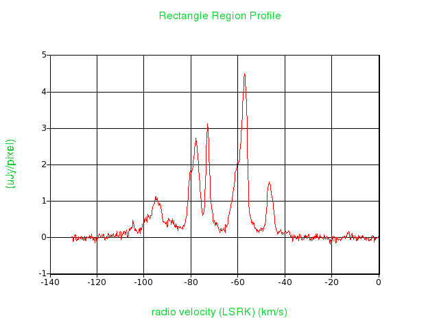
Figure 3: a spectral profile in the box marked in green
Input: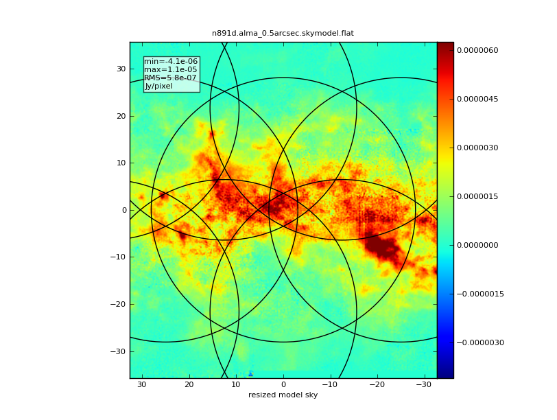
|
Predict:
|
Image: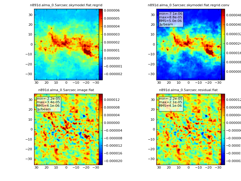
|
Analyze: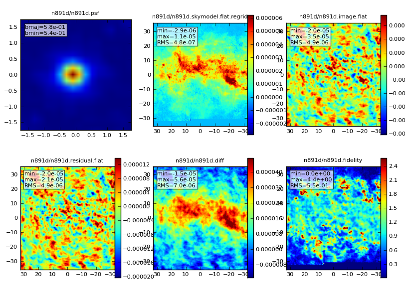
|
Figure 4: Sample results
Last checked on CASA Version 3.4.0.