NGC3256 Band3 Calibration for CASA 3.4
Overview
This portion of the NGC3256Band3 CASA Guide will cover the calibration of the raw visibility data. To skip to the imaging portion of the guide, see: NGC3256 Band3 - Imaging.
If you haven't already downloaded the raw data, you may do that now by clicking on the region closest to your location and downloading the file named 'NGC3256_Band3_UnCalibratedMSandTablesForReduction.tgz':
Once the download has finished, unpack the file:
# In a terminal outside CASA
tar -xvzf NGC3256_Band3_UnCalibratedMSandTablesForReduction.tgz

cd NGC3256_Band3_UnCalibratedMSandTablesForReduction

# Start CASA
casapy
The data have already been converted to CASA Measurement Set (MS) format using the CASA task importasdm. Accompanying the data are some basic calibration tables you will need for the following reduction, as well as the *.ms.flagversions files that are automatically generated by importasdm.
Initial Inspection and A priori Flagging
We will eventually concatenate the six datasets used here into one large dataset. However, we will keep them separate for now, as some of the steps to follow require individual datasets (specifically, the application of the Tsys and WVR tables). We therefore start by defining an array "basename" that includes the names of the six files in chronological order. This will simplify the following steps by allowing us to loop through the files using a simple for-loop in python. Remember that if you log out of CASA, you will have to re-issue this command. We will remind you of this in the relevant sections by repeating the command at the start.
# In CASA
basename=['uid___A002_X1d54a1_X5','uid___A002_X1d54a1_X174','uid___A002_X1d54a1_X2e3',
'uid___A002_X1d5a20_X5','uid___A002_X1d5a20_X174','uid___A002_X1d5a20_X330']
The usual first step is then to get some basic information about the data. We do this using the task listobs, which will output a detailed summary of each dataset supplied.
# In CASA
for name in basename:
        listobs(vis=name+'.ms')
Note that after cutting and pasting a for-loop you often have to press return several times to execute. The output will be sent to the CASA logger. You will have to scroll up to see the individual output for each of the six datasets. Here is an example of the most relevant output for the first file in the list.
	Fields: 3
	  ID   Code Name                RA              Decl          Epoch   SrcId nRows
	  0    none 1037-295            10:37:16.07900 -29.34.02.8130 J2000   0     38759
	  1    none Titan               00:00:00.00000 +00.00.00.0000 J2000   1     16016
	  2    none NGC3256             10:27:51.60000 -43.54.18.0000 J2000   2     151249
	Spectral Windows:  (9 unique spectral windows and 2 unique polarization setups)
	  SpwID  #Chans Frame Ch1(MHz)    ChanWid(kHz)  TotBW(kHz)  Corrs
	  0           4 TOPO  184550      1500000       7500000     I
	  1         128 TOPO  113211.988  15625         2000000     XX  YY
	  2           1 TOPO  114188.55   1796875       1796875     XX  YY
	  3         128 TOPO  111450.813  15625         2000000     XX  YY
	  4           1 TOPO  112427.375  1796875       1796875     XX  YY
	  5         128 TOPO  101506.187  15625         2000000     XX  YY
	  6           1 TOPO  100498.375  1796875       1796875     XX  YY
	  7         128 TOPO  103050.863  15625         2000000     XX  YY
	  8           1 TOPO  102043.05   1796875       1796875     XX  YY
	Sources: 48
	  ID   Name                SpwId RestFreq(MHz)  SysVel(km/s)
	  0    1037-295            0     -              -
	  0    1037-295            9     -              -
	  0    1037-295            10    -              -
	  0    1037-295            11    -              -
	  0    1037-295            12    -              -
	  0    1037-295            13    -              -
	  0    1037-295            14    -              -
	  0    1037-295            15    -              -
	  0    1037-295            1     -              -
	  0    1037-295            2     -              -
	  0    1037-295            3     -              -
	  0    1037-295            4     -              -
	  0    1037-295            5     -              -
	  0    1037-295            6     -              -
	  0    1037-295            7     -              -
	  0    1037-295            8     -              -
	  1    Titan               0     -              -
	  1    Titan               9     -              -
	  1    Titan               10    -              -
	  1    Titan               11    -              -
	  1    Titan               12    -              -
	  1    Titan               13    -              -
	  1    Titan               14    -              -
	  1    Titan               15    -              -
	  1    Titan               1     -              -
	  1    Titan               2     -              -
	  1    Titan               3     -              -
	  1    Titan               4     -              -
	  1    Titan               5     -              -
	  1    Titan               6     -              -
	  1    Titan               7     -              -
	  1    Titan               8     -              -
	  2    NGC3256             0     -              -
	  2    NGC3256             9     -              -
	  2    NGC3256             10    -              -
	  2    NGC3256             11    -              -
	  2    NGC3256             12    -              -
	  2    NGC3256             13    -              -
	  2    NGC3256             14    -              -
	  2    NGC3256             15    -              -
	  2    NGC3256             1     -              -
	  2    NGC3256             2     -              -
	  2    NGC3256             3     -              -
	  2    NGC3256             4     -              -
	  2    NGC3256             5     -              -
	  2    NGC3256             6     -              -
	  2    NGC3256             7     -              -
	  2    NGC3256             8     -              -
	Antennas: 7:
	  ID   Name  Station   Diam.    Long.         Lat.
	  0    DV04  J505      12.0 m   -067.45.18.0  -22.53.22.8
	  1    DV06  T704      12.0 m   -067.45.16.2  -22.53.22.1
	  2    DV07  J510      12.0 m   -067.45.17.8  -22.53.23.5
	  3    DV08  T703      12.0 m   -067.45.16.2  -22.53.23.9
	  4    DV09  N602      12.0 m   -067.45.17.4  -22.53.22.3
	  5    PM02  T701      12.0 m   -067.45.18.8  -22.53.22.2
	  6    PM03  J504      12.0 m   -067.45.17.0  -22.53.23.0
This output shows that three fields were observed: 1037-295, Titan, and NGC3256. Field 0 (1037-295) will serve as the gain calibrator and bandpass calibrator; field 1 (Titan) will serve as the flux calibrator; and field 2 (NGC3256) is, of course, the science target.
Note that there are more than four SpwIDs even though the observations were set up to have four spectral windows. The spectral line data themselves are found in spectral windows 1,3,5,7, which have 128 channels each. The first one (spw 1) is centered on the CO(1-0) emission line in the galaxy NGC 3256 and is our highest frequency spectral window. There is one additional spectral window (spw 3) in the Upper Side Band (USB), and there are two spectral windows (spw 5 and 7) in the Lower Side Band (LSB). These additional spectral windows are used to measure the continuum emission in the galaxy, and may contain other emission lines as well.
Spectral windows 2,4,6,8 contain channel averages of the data in spectral windows 1,3,5,7, respectively. These are not useful for the offline data reduction. Spectral window 0 contains the WVR data. You may notice that there are additional SpwIDs listed in the "Sources" section which are not listed in the "Spectral Windows" section. These spectral windows are reserved for the WVRs of each antenna (seven in our case). At the moment, all WVRs point to spw 0, which contains nominal frequencies. The additional spectral windows (spw 9-15) are therefore not used and can be ignored.
Another important thing to note is that the position of Titan is listed as 00:00:00.0000 +00.00.00.0000. This is due to the fact that for ephemeris objects, the positions are currently not stored in the asdm. This will be handled correctly in the near future, but at present, we have to fix this offline. We will correct the coordinates below by running the procedure fixplanets, which takes the position from the pointing table.
The final column of the listobs output in the logger (not shown above) gives the scan intent. This information is used later to flag the pointing scans and the hot and ambient load calibration scans, using scan intent as a selection option. Also these intents will be used in the future for pipeline processing.
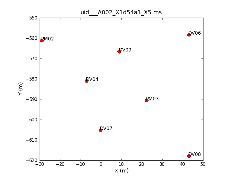
Seven antennas were used for the dataset listed above. Note that numbering in python always begins with "0", so the antennas have IDs 0-6. To see what the antenna configuration looked like at the time of the this observation, we will use the task plotants.

# In CASA
plotants(vis=basename[0]+'.ms', figfile=basename[0]+'_plotants.png')
This will plot the antenna configuration on your screen as well as save it under the specified filename for future reference. This will be important later on when we need to choose a reference antenna, since the reference antenna should be close to the center of the array (as well as stable and present for the entire observation).
If you repeat the plotants command for the other five datasets, you will see that there is an additional antenna (DV10) present on the second day of observations. Other than that, the configuration stays constant during the course of the observations.
Flagging
The first editing we will do is some a priori flagging with tflagdata. We will start by flagging the shadowed data and the autocorrelation data. ALMA data contains both the cross correlation and autocorrelation data, but here we are only interested in the cross-correlation data. Additionally, for compact configurations of the array, one antenna can shadow another, blocking its view. These data also need to be flagged.
There are a number of scans in the data that were used by the online system for pointing calibration. These scans are no longer needed, and we can flag them easily with tflagdata by selecting on 'intent'.
Remember that you first need to redefine the "basename" array if you logged out of CASA prior to starting this section.
# In CASA
basename=['uid___A002_X1d54a1_X5','uid___A002_X1d54a1_X174','uid___A002_X1d54a1_X2e3',
'uid___A002_X1d5a20_X5','uid___A002_X1d5a20_X174','uid___A002_X1d5a20_X330']
Now we will loop over the datasets, running the flagging commands:
# In CASA
for name in basename:
	tflagdata(vis=name+'.ms', mode='shadow', applyflags=T, flagbackup = F, async=False)

for name in basename:
        default(tflagdata)
        vis=name+'.ms'
	applyflags=T
	flagbackup = T
	async=False
        mode='manual'
	intent='*POINTING*'
        tflagdata()
	intent='*ATMOSPHERE*'
        tflagdata()
	intent=''
        antenna='*&&&'
        tflagdata()
We will then store the current flagging state for each dataset using the flagmanager:
# In CASA
for name in basename:
        flagmanager(vis = name+'.ms', mode = 'save', versionname = 'Apriori')
Delay Correction (mainly for Antenna DV07)
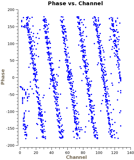
Due to an issue with antenna DV07 during the commissioning period when these data were taken, it shows large delays in phase for the first three datasets. While the bandpass calibration will attempt to fit and remove small phase delays (i.e., less than one wrap over the bandpass), large delays like those seen here will result in failed solutions. If we want to salvage the data for this antenna, we therefore need to correct the delays by calculating a K-type delay calibration table with gencal. We emphasize that this is not usually a part of the typical calibration procedure, but it may be useful to the reader to see how such a correction is made.
Remember that you first need to redefine the "basename" array if you logged out of CASA prior to starting this section.
# In CASA
basename=['uid___A002_X1d54a1_X5','uid___A002_X1d54a1_X174','uid___A002_X1d54a1_X2e3',
'uid___A002_X1d5a20_X5','uid___A002_X1d5a20_X174','uid___A002_X1d5a20_X330']

You can see the phase delays by plotting phase versus channel in plotms, as we do here for a single spw, correlation, and baseline with DV07:
# In CASA
plotms(vis=basename[0]+'.ms', xaxis='channel', yaxis='phase',
        spw='3', antenna='PM03&DV07', correlation='XX', avgtime='1e8')
We run gaincal on all datasets, which yields a delay correction for all antennas. This will remove the phase wrapping and seen on baselines incolving DV07. and will aslo serve as a first phase calibration for all baselines. As the gaincal task will not overwrite existing tables, the script starts by deleting any existing versions of the calibration tables with the same name.


# In CASA
for name in basename:
	os.system('rm -rf cal-'+name+'_del.K')
	gaincal(vis=name+'.ms', caltable='cal-'+name+'_del.K',
		field="1037*",spw="1:10~120,3:10~120,5:10~120,7:10~120",
		solint="inf",combine="scan",refant="DV04",
		gaintype="K")
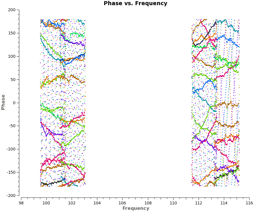
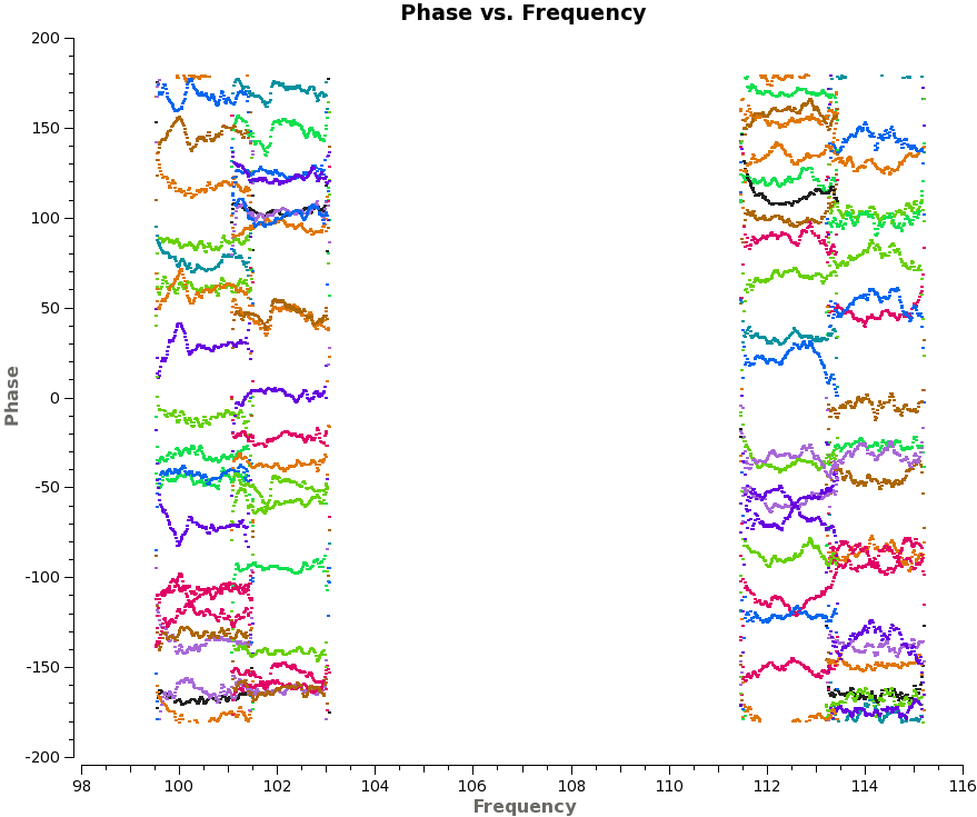
We will apply these K tables to the data in the next section together with the WVR and Tsys correction. To visualize the effect that the delay correction has you may apply the calibration, and then plot first the uncorrected data, and then the corrected data (by selecting 'corrected' in the axes - Y axis - data column field in the plotms GUI). The phase wrapping apparent on a number of baselines should have dissapeared, and the phases should not show large drifts anymore:
# In CASA
for name in basename:
         applycal(vis=name+'.ms', flagbackup=F, spw='1,3,5,7',
         interp='nearest', gaintable='cal-'+name+'_del.K')

plotms(vis=basename[0]+'.ms', xaxis='freq', yaxis='phase',
         spw='1,3,5,7', antenna='', correlation='XX', avgtime='1e8',
         coloraxis='baseline', avgscan=T, selectdata=T, field='1037*')