Calibrating a Mosaicked Spectral Line Dataset: Difference between revisions
No edit summary |
No edit summary |
||
| Line 17: | Line 17: | ||
</source> | </source> | ||
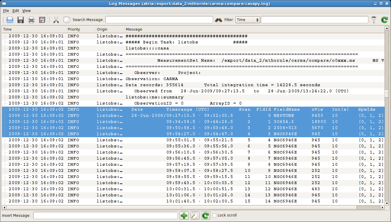
You will want to know: | You will want to know: [[Image:listobs1a.png | thumb| The beginning of the output from listobs.]] | ||
* The FieldId of each of your sources and calibrators. | * The FieldId of each of your sources and calibrators. | ||
| Line 23: | Line 23: | ||
* The Name (or station, but ''not'' the ID ) of your reference antenna. | * The Name (or station, but ''not'' the ID ) of your reference antenna. | ||
Near the beginning of the listobs output, you will find the first listing of FldId numbers. In this case, the flux calibrator (NEPTUNE) is assigned FldId=0, the bandpass calibrator (3C454.3) is assigned FldId=1, the phase calibrator (2038+513) is assigned FldId=2, and the mosaicked source fields are assigned FldId 3 through 51 (that's field='3~51' in python). | Near the beginning of the listobs output, you will find the first listing of FldId numbers. In this case, the flux calibrator (NEPTUNE) is assigned FldId=0, the bandpass calibrator (3C454.3) is assigned FldId=1, the phase calibrator (2038+513) is assigned FldId=2, and the mosaicked source fields are assigned FldId 3 through 51 (that's field='3~51' in python). | ||
| Line 38: | Line 37: | ||
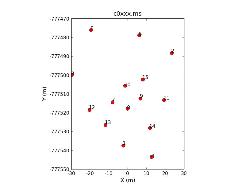
will display the physical layout of the antennas.[[Image:plotxyexample.png|thumb|plotxy output showing antenna positions. ]] You can see ANT 8 near the middle of the CARMA array. | will display the physical layout of the antennas.[[Image:plotxyexample.png|thumb|plotxy output showing antenna positions. ]] You can see ANT 8 near the middle of the CARMA array. | ||
== Calibrating your data == | |||
Before running your calibration, it's a good idea to run the following command: | |||
<source lang="python"> | |||
# In CASA | |||
clearcal(vis=msfile) | |||
</source> | |||
If this is the first time you've calibrated, clearcal won't do much, but it will initialize table format that might be missing from the import step. If you are trying a new calibration, this command ensures your data returns to their original state. So it can't hurt you, and can help. | |||
=== Bandpass calibration === | |||
<source lang="python"> | |||
# In CASA | |||
default('bandpass') | |||
bandpass(vis=catfile,caltable=msdir+proj+'.bcal',gaintable='',gainfield='', | |||
interp='',field='1',spw='',gaincurve=False, | |||
bandtype='B',solint='inf',refant='ANT8', | |||
solnorm=True) | |||
</source> | |||
=== Amplitude calibration === | |||
<source lang="python"> | |||
# In CASA | |||
setjy(vis=catfile, field='1',fluxdensity=[6.6,0.,0.,0.], spw='0~2') | |||
</source> | |||
<source lang="python"> | |||
# In CASA | |||
gaincal(vis=catfile,caltable=msdir+proj+'.gcal',gaintable=msdir+proj+'.bcal', | |||
gainfield='1', field='1,2', spw='0', | |||
gaintype='G',minsnr=2.0, refant='ANT8', solint='inf', combine='') | |||
</source> | |||
<source lang="python"> | |||
# In CASA | |||
</source> | |||
Revision as of 15:57, 28 December 2009
This page assumes you have converted your data from native MIRIAD format to a CASA measurement set (MS). It also assumes that you have put the filename of the original MS into a global CASA variable, e.g.,
# In CASA
project='c0xxx'
msfile=project+'.ms'
Examining your data
You'll need some information about the IDs that CASA assigns to your calibrators, sources, and antennas. So if you haven't yet done so,
# In CASA
listobs(vis=msfile)
You will want to know:

- The FieldId of each of your sources and calibrators.
- The SpwId of each spectral window you want to calibrate.
- The Name (or station, but not the ID ) of your reference antenna.
Near the beginning of the listobs output, you will find the first listing of FldId numbers. In this case, the flux calibrator (NEPTUNE) is assigned FldId=0, the bandpass calibrator (3C454.3) is assigned FldId=1, the phase calibrator (2038+513) is assigned FldId=2, and the mosaicked source fields are assigned FldId 3 through 51 (that's field='3~51' in python).
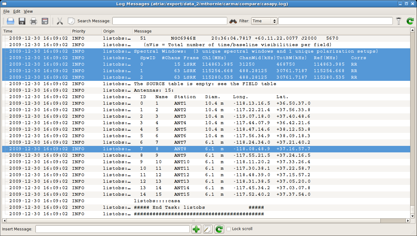
Near the end of the listobs output, you will find listings of the properties of the observed spectral windows, and the locations of the antennas. In this case, the narrowband windows are assigned to SpwID of 1 and 2, and they each have 63 channels. The reference antenna is Antenna 8, which unfortunately here is named '8'. For unambiguous antenna selection, ideally the Name (which CASA searches first) should have text in it; if it does not, you may want to use the unambiguous Station name of 'ANT8' to ensure that CASA chooses the right antenna.

It's not particularly clear, without a closer look at this output, which antenna you should use as the reference antenna. You can get this information using plotxy. The following command
# In CASA
plotxy(vis=msfile,xaxis='x')
will display the physical layout of the antennas.

You can see ANT 8 near the middle of the CARMA array.
Calibrating your data
Before running your calibration, it's a good idea to run the following command:
# In CASA
clearcal(vis=msfile)
If this is the first time you've calibrated, clearcal won't do much, but it will initialize table format that might be missing from the import step. If you are trying a new calibration, this command ensures your data returns to their original state. So it can't hurt you, and can help.
Bandpass calibration
# In CASA
default('bandpass')
bandpass(vis=catfile,caltable=msdir+proj+'.bcal',gaintable='',gainfield='',
         interp='',field='1',spw='',gaincurve=False,
         bandtype='B',solint='inf',refant='ANT8',
         solnorm=True)
Amplitude calibration
# In CASA
setjy(vis=catfile, field='1',fluxdensity=[6.6,0.,0.,0.], spw='0~2')
# In CASA
gaincal(vis=catfile,caltable=msdir+proj+'.gcal',gaintable=msdir+proj+'.bcal',
        gainfield='1', field='1,2', spw='0',
        gaintype='G',minsnr=2.0, refant='ANT8', solint='inf', combine='')
# In CASA