N891 simdata (CASA 3.3): Difference between revisions
No edit summary |
No edit summary |
||
| Line 24: | Line 24: | ||
</source> | </source> | ||
Units: K - first convert to flux surface brightness: Jy/Sr = 2x10<sup>23</sup> k T / λ<sup>2</sup>, | |||
<!-- <math>\frac{Jy}{Sr} = \frac{2\times 10^{23} k T}{\pi D^2 \Omega}</math>, where <math>\Omega</math> is the beam solid angle --> | <!-- <math>\frac{Jy}{Sr} = \frac{2\times 10^{23} k T}{\pi D^2 \Omega}</math>, where <math>\Omega</math> is the beam solid angle --> | ||
= 4x10<sup>8</sup>T at 110GHz. | = 4x10<sup>8</sup>T at 110GHz. | ||
<source lang="python"> | <source lang="python"> | ||
# In CASA | |||
# Setting the new frequency of the central channel | # Setting the new frequency of the central channel | ||
incenter = "110.1777GHz" | incenter = "110.1777GHz" | ||
| Line 34: | Line 35: | ||
* Now we need to decide if this model data will work at the desired pixel scale | * Now we need to decide if this model data will work at the desired pixel scale | ||
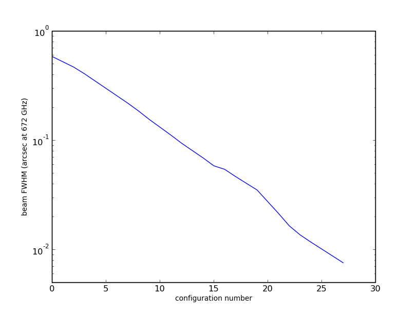
* the GRS resolution of 40" at ~10kpc is 0.04" at 10Mpc, so we should be able to do a simulation of observing at ~0.1-0.2". The resolution plot (See Figure 1) indicates that for ALMA at 100GHz, configuration 20 is appropriate. | |||
[[Image:Beamsummary.png|thumb|Figure 1: Resolution plot.]] | [[Image:Beamsummary.png|thumb|Figure 1: Resolution plot.]] | ||
* If we intend to set <tt>cell=0.04arcsec</tt> in <tt>simdata</tt>, then the cube needs to be multiplied by 4x10<sup>8</sup> * (.04/206265)<sup>2</sup> = 1.4x10<sup>-5</sup> to obtain Jy/pixel. The cube peaks at ~20K, so we can perform the simulation with <tt>inbright=3e-4</tt>, which should yield a peak of ~1mJy/bm. | |||
4x10<sup>8</sup> * (.04/206265)<sup>2</sup> = 1.4x10<sup>-5</sup> to obtain Jy/pixel. The cube peaks at ~20K, so we can perform the simulation with <tt>inbright=3e-4</tt>, which should yield a peak of ~1mJy/bm. | |||
* Will we be dominated by the noise in the input model? | |||
Input noise ~150mK or S/N~20, so at our scaled intensity, ~0.05 mJy/bm. The [http://www.eso.org/sci/facilities/alma/observing/tools/etc/ exposure time calculator] says that ALMA will achieve 2.5mJy/bm in 2 hours for the input 212m/s channel width (0.075MHz), so the noise in the input model should not affect our results. | |||
<source lang="python"> | |||
# In CASA | |||
# Setting the new channel width | |||
inwidth = "0.075MHz" | |||
</source> | |||
* We do have a sensitivity issue though - if we decrease the spectral resolution by a factor of 6 (bin the input channels in some other program - simdata will know how to do that in the future but not yet), and plan for 3 8-hr tracks, then the sensitivity calculator suggests that we'll get <0.25mJy rms, or S/N>10 per beam. Rather than simulate 3 days of observing, I'll increase inbright by sqrt(3) and simulate one 8 hour track. | * We do have a sensitivity issue though - if we decrease the spectral resolution by a factor of 6 (bin the input channels in some other program - simdata will know how to do that in the future but not yet), and plan for 3 8-hr tracks, then the sensitivity calculator suggests that we'll get <0.25mJy rms, or S/N>10 per beam. Rather than simulate 3 days of observing, I'll increase inbright by sqrt(3) and simulate one 8 hour track. | ||
<source lang="python"> | |||
# In CASA | |||
# Scaling the surface brightness | |||
inbright = "1.4e-4" | |||
</source> | |||
setup: | setup: | ||
* the ALMA 12m primary beam is 50" so we'd space a mosaic by 25", but the model cube has 326x357 pixels, or 13 arcsec with our small pixels. That's a lot smaller than the primary beam, so it doesn't matter much what output image size we ask for. | * the ALMA 12m primary beam is 50" so we'd space a mosaic by 25", but the model cube has 326x357 pixels, or 13 arcsec with our small pixels. That's a lot smaller than the primary beam, so it doesn't matter much what output image size we ask for. | ||
<source lang="python"> | |||
# In CASA | |||
# Finish up the image model, and setting up the pointing | |||
indirection = 'J2000 7h00m34 -23d03m00' | indirection = 'J2000 7h00m34 -23d03m00' | ||
incell = "0.2arcsec" | incell = "0.2arcsec" | ||
| Line 57: | Line 67: | ||
pointingspacing = "25arcsec" | pointingspacing = "25arcsec" | ||
mapsize = '60arcsec' | mapsize = '60arcsec' | ||
</source> | |||
There are 659 channels in the input cube, but as noted above we want to bin those to 109 channels of 1.2 km/s each. | |||
<source lang="python"> | |||
#In CASA | |||
graphics = "both" | graphics = "both" | ||
verbose = True | verbose = True | ||
Revision as of 19:21, 3 October 2011
↵ Simulating Observations in CASA
Old version: N891 simdata2.
To create a script of the Python code on this page see Extracting scripts from these tutorials.
Nearby edge-on spiral
Roughly modeled after NGC891
This article is under construction. Watch this space!
- mostly correct, but probably not very thoroughly explained. Updated for CASA 3.3
- model origin: Milky Way 13CO from the Galactic Ring Survey on the 14m FCRAO
- I binned the cube to coarser velocity resolution in order to speed the simulation. the fits file is grs-12kms.fits
# In CASA
# Initializing simdata
# Laying down some basic ground rules
default("simdata")
project            =  "n891d"
skymodel         =  "grs-12kms.fits"
Units: K - first convert to flux surface brightness: Jy/Sr = 2x10²³ k T / λ2, = 4x10⁸T at 110GHz.
# In CASA
# Setting the new frequency of the central channel
incenter          =  "110.1777GHz"
- Now we need to decide if this model data will work at the desired pixel scale
- the GRS resolution of 40" at ~10kpc is 0.04" at 10Mpc, so we should be able to do a simulation of observing at ~0.1-0.2". The resolution plot (See Figure 1) indicates that for ALMA at 100GHz, configuration 20 is appropriate.
- If we intend to set cell=0.04arcsec in simdata, then the cube needs to be multiplied by 4x108 * (.04/206265)2 = 1.4x10⁻⁵ to obtain Jy/pixel. The cube peaks at ~20K, so we can perform the simulation with inbright=3e-4, which should yield a peak of ~1mJy/bm.
- Will we be dominated by the noise in the input model?
Input noise ~150mK or S/N~20, so at our scaled intensity, ~0.05 mJy/bm. The exposure time calculator says that ALMA will achieve 2.5mJy/bm in 2 hours for the input 212m/s channel width (0.075MHz), so the noise in the input model should not affect our results.
# In CASA
# Setting the new channel width
inwidth          =  "0.075MHz"
- We do have a sensitivity issue though - if we decrease the spectral resolution by a factor of 6 (bin the input channels in some other program - simdata will know how to do that in the future but not yet), and plan for 3 8-hr tracks, then the sensitivity calculator suggests that we'll get <0.25mJy rms, or S/N>10 per beam. Rather than simulate 3 days of observing, I'll increase inbright by sqrt(3) and simulate one 8 hour track.
# In CASA
# Scaling the surface brightness
inbright           =  "1.4e-4"
setup:
- the ALMA 12m primary beam is 50" so we'd space a mosaic by 25", but the model cube has 326x357 pixels, or 13 arcsec with our small pixels. That's a lot smaller than the primary beam, so it doesn't matter much what output image size we ask for.
# In CASA
# Finish up the image model, and setting up the pointing
indirection          =  'J2000 7h00m34 -23d03m00'
incell               =  "0.2arcsec"
setpointings = True
integration        =  "300s"
pointingspacing    =  "25arcsec"
mapsize = '60arcsec'
There are 659 channels in the input cube, but as noted above we want to bin those to 109 channels of 1.2 km/s each.
#In CASA
graphics = "both"
verbose = True
overwrite = True
observe = True
antennalist        =  "alma;0.5arcsec"
totaltime          =  "3600s"
image=T
simdata()
here's the cube with the simdata's scaling and World Coordinate System:
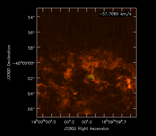
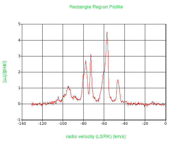
and a spectral profile in the box marked in green
Sample results:
Input: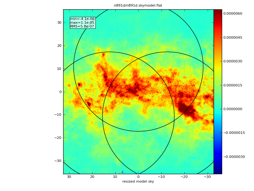
|
Predict: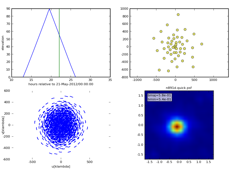
|
Image: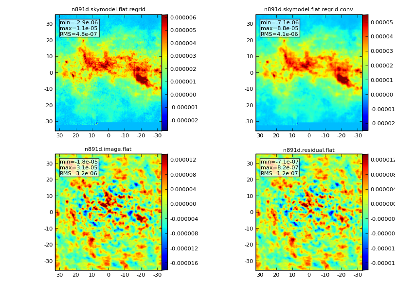
|
Analyze: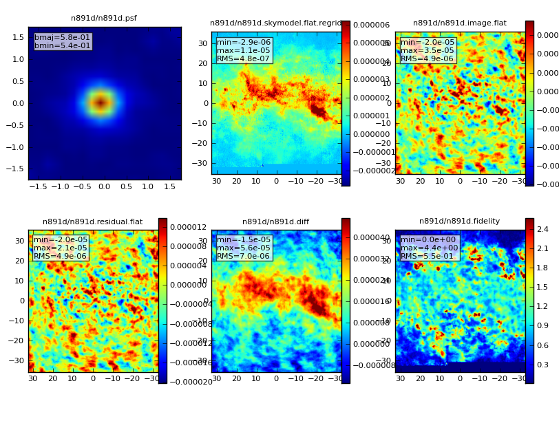
|