PPdisk simdata (CASA 3.3)

↵ Simulating Observations in CASA

Old version: PPdisk simdata (CASA 3.2).

To create a script of the Python code on this page see Extracting scripts from these tutorials.

Protoplanetary disk

• This fits file is a model of a protoplanetary disk from S. Wolf (If you use it for anything more than learning CASA, please cite Wolf & D'Angelo 2005).

• Simdata version for CASA 3.2

Explanation of the script

Set simdata as current task and reset all parameters

# Setting everything in simdata to original defaults
default("simdata")

Specify sky model image

# Prior image to use in clean
# Make sure you are running CASA in the same directory as this file
modelimage         =  "input50pc_672GHz.fits"

Image coordinate system can be verified

# This reports image header parameters in the Log Messages window
imhead("input50pc_672GHz.fits")

Image center can be identified

# These are tools found in the CASA toolkit
# They are very useful, but the interface is not as straightforward as the tasks
# You can find the tool reference manual here: http://casa.nrao.edu/docs/CasaRef/CasaRef.html
# The following command is used to open an image (this is part of the image analysis toolkit)
# Whenever data are being viewed/manipulated by tools, what is being operated on needs to be explicitly opened
# and closed (i.e. an image, a table, etc.)
ia.open("input50pc_672GHz.fits")
#  Out[9]: True
# Reports the length of each axis in the opened image
ia.shape()
#  Out[11]: [257L, 257L, 1L, 1L]
# This command converts from pixel (our source file) to world coordinate (something usable by simdata)
ia.toworld([128.5,128.5])
#  Out[12]:
#{'numeric': array([  4.71239120e+00,  -4.01423802e-01,   1.00000000e+00,
#         6.72000001e+11])}
# Formats the coordinate just converted into hms
qa.formxxx("4.71239120rad",format='hms',prec=5)
#  Out[13]: '18:00:00.03052'
# Formats one of the other coordinates into dms
qa.formxxx("-0.401423802rad",format='dms',prec=5)
#  Out[14]: '-022.59.59.602743'
# Final housekeeping by closing the image tool
# The image tool is now detached from the image
ia.close()

Brightness scale can be viewed with 'imstat' task

# Default parameters are adequate for this
imstat("input50pc_672GHz.fits")
# ...
#  'max': array([  6.52469971e-05]),
# ...
# that's 0.0652 mJy/pixel.

Let's call our project psim2

# This defines the root prefix for any output files from simdata
project            =  "psim2"

We'll leave the sky model the way it is: simdata will create psim2.skymodel CASA image since this model is a fits file, and most but not all of CASA routines can operate directly on fits

skymodel           =  "input50pc_672GHz.fits"

We need to decide where to point the telescope. The image is 2/3 arcsec in size, so we only need one pointing. We could put that in a text file ourself, or let simdata create the ascii pointing file for us.

setpointings       =  True
direction          =  "J2000 18h00m00.031s -22d59m59.6s"
mapsize            =  "0.76arcsec"

We do want to calculate visibilities in a measurement set: let's do a 20 min snapshot observation using the "out20" ALMA antenna configuration:

observe            =  True
totaltime          =  "1200s"

Use appropriate antenna configurations based on desired angular resolution (configuration 20 - alma.out20.cfg in this case - is the largest "compact" configuration)

# It might be helpful to confirm the alma.out20.cfg file exists in the path defined below
# If you have a problem, this might be the first thing to check, if you haven't already
repodir=os.getenv("CASAPATH").split(' ')[0]
antennalist        =  repodir+"/data/alma/simmos/alma.out20.cfg"

Deconvolve the visibilities back into an image

image              =  True
vis                =  "$project.ms"
imsize             =  [192, 192]

Specify number of iteration of cleaning task with proper threshold and weighting

niter              =  10000
threshold          =  "1e-7Jy"
weighting          =  "natural"

We'd like to calculate a difference and fidelity image, and see some diagnostics:

analyze            =  True

And see the array but not the UV coverage:

showarray          =  True
showuv             =  False

Plot both to the screen and the png files with lots of messages:

graphics           =  "both"
verbose            =  True
overwrite = True

Run simdata

# This commands CASA to execute simdata
simdata()

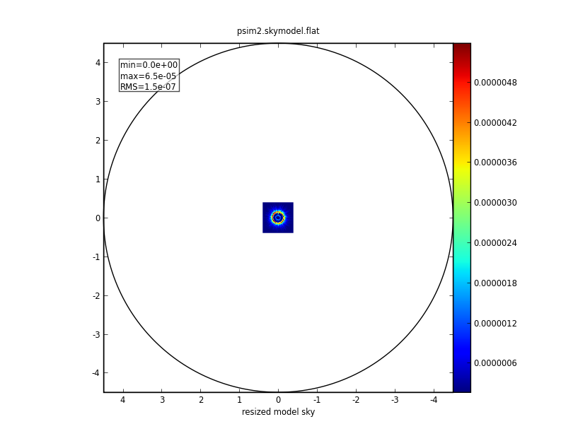
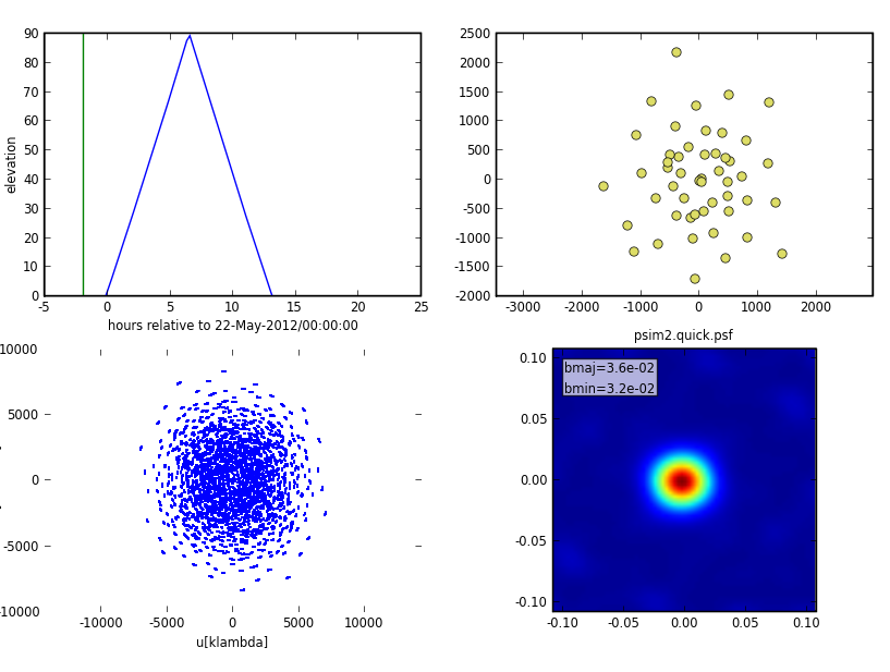
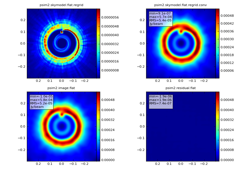
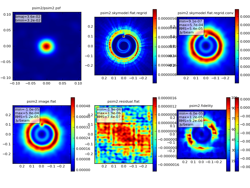
• Output results:

Input:	Predict:
Image:	Analyze:

↵ Simulating Observations in CASA