EVLA 6cmWideband Tutorial SN2010FZ: Difference between revisions
| Line 966: | Line 966: | ||
=== Cleaning using both basebands combined === | === Cleaning using both basebands combined === | ||
For the ultimate image, use the "clean" part of the upper baseband in addition | |||
to the lower (use spw 0-11). We will use mfs with nterms=2 (if you try nterms=1 | |||
on this wide bandwidth you will get much poorer residuals). | |||
<source lang="python"> | <source lang="python"> | ||
# In CASA | # In CASA | ||
| Line 980: | Line 982: | ||
print 'Residual standard deviation = '+str(mystat['sigma'][0]) | print 'Residual standard deviation = '+str(mystat['sigma'][0]) | ||
</source> | </source> | ||
I got 8.2uJy. | I got 8.2uJy. | ||
Look at this in the viewer: | Look at this in the viewer: | ||
Revision as of 14:59, 30 August 2011
Overview
This article describes the calibration and imaging of a single-pointing 6cm EVLA wideband continuum dataset on the galaxy NGC2967 (UGC5180) which was the location of the supernova candidate SN2010FZ. No supernova was detected in this observation, but the galactic continuum emission from this face-on spiral is adequately imaged. The data were taken in RSRO mode, with 1024 MHz of bandwidth in each of two widely spaced basebands (comprised each of 8 128 MHz spectral windows), spanning 4.5 to 7.5 GHz. We will use wideband imaging techniques in this tutorial.
This is a more advanced tutorial, and if you are a relative novice (and particularly for EVLA continuum calibration and imaging), it is strongly recommended that you start with the EVLA Continuum Tutorial 3C391 before tackling this dataset. We will not include basic information on CASA processing in this tutorial.
CASA Versions
This tutorial was written for the CASA Version 3.2.1 (release r15198 26 May 2011).
Obtaining the Data
The scheduling block (SB) processed appears in the EVLA archive under program AS1015 as AS1015_sb1658169_1.55388.89474846065 and was run on 2010-07-11 from 21:28 to 22:28 UT (size 37.74GB).
For the purposes of this tutorial, we have provided the raw SDM data (as would be extracted from the archive) as well as measurement sets created by filling the data (with the importevla task) and upon time-averaging to 10s (after application of the online flags).
To start your tutorial, depending on which dataset you start with, proceed to:
- To start with the raw SDM data: Start with the section below titled "#Importing your EVLA data from SDM". This is where you would start if you were reducing data from the archive.
- To start with the raw filled MS: Start with the section below titled "#Application of Online Flags and Averaging your MS".
- To start with the flagged and averaged MS: Start with the section below titled "#Examining and Flagging your Averaged MS".
Importing your EVLA data from SDM
For the purposes of this tutorial, we assume that the SDM is resident on disk, in this case at the location:
/lustre/smyers/AS1015/AS1015_sb1658169_1.55388.89474846065
Use the actual location of your data when you carry out the commands.
The listsdm task will print out a summary of the scans, fields, spectral windows, and antennas present in your SDM.
# In CASA
listsdm('/lustre/smyers/AS1015/AS1015_sb1658169_1.55388.89474846065')
In the logger you should see:
================================================================================
   SDM File: /lustre/smyers/AS1015/AS1015_sb1658169_1.55388.89474846065
================================================================================
   Observer: Dr. Alicia M. Soderberg
   Facility: EVLA, D-configuration
      Observed from 2010/07/11/21:28:28.41 to 2010/07/11/22:28:17.73 (UTC)
      Total integration time = 3589.32 seconds (1.00 hours)

Scan listing:
  Timerange (UTC)           Scan FldID  FieldName       SpwIDs         Intent(s)
  21:28:28.41 - 21:29:27.40    1     0  J0925+0019      [0, 1]  CALIBRATE_PHASE
  21:29:27.40 - 21:30:57.16    2     0  J0925+0019      [0, 1]  CALIBRATE_PHASE
  21:30:57.16 - 21:32:26.91    3     0  J0925+0019      [0, 1]  CALIBRATE_PHASE
  21:32:26.91 - 21:33:56.67    4     0  J0925+0019      [0, 1]  CALIBRATE_PHASE
  21:33:56.67 - 21:34:56.50    5     0  J0925+0019      [0, 1]  CALIBRATE_PHASE
  21:34:56.50 - 21:35:56.34    6     0  J0925+0019      [2, 3, 4, 5, 6, 7, 8, 9, 10, 11, 12, 13, 14, 15, 16, 17]  CALIBRATE_PHASE
  21:35:56.34 - 21:37:26.09    7     0  J0925+0019      [2, 3, 4, 5, 6, 7, 8, 9, 10, 11, 12, 13, 14, 15, 16, 17]  CALIBRATE_PHASE
  21:37:26.09 - 21:38:25.93    8     0  J0925+0019      [2, 3, 4, 5, 6, 7, 8, 9, 10, 11, 12, 13, 14, 15, 16, 17]  CALIBRATE_PHASE
  21:38:25.93 - 21:39:55.68    9     1  SN2010FZ        [2, 3, 4, 5, 6, 7, 8, 9, 10, 11, 12, 13, 14, 15, 16, 17]  OBSERVE_TARGET
  21:39:55.68 - 21:41:25.44   10     1  SN2010FZ        [2, 3, 4, 5, 6, 7, 8, 9, 10, 11, 12, 13, 14, 15, 16, 17]  OBSERVE_TARGET
  21:41:25.44 - 21:42:55.19   11     1  SN2010FZ        [2, 3, 4, 5, 6, 7, 8, 9, 10, 11, 12, 13, 14, 15, 16, 17]  OBSERVE_TARGET
  21:42:55.19 - 21:44:24.94   12     1  SN2010FZ        [2, 3, 4, 5, 6, 7, 8, 9, 10, 11, 12, 13, 14, 15, 16, 17]  OBSERVE_TARGET
  21:44:24.94 - 21:45:54.70   13     1  SN2010FZ        [2, 3, 4, 5, 6, 7, 8, 9, 10, 11, 12, 13, 14, 15, 16, 17]  OBSERVE_TARGET
  21:45:54.70 - 21:47:24.45   14     1  SN2010FZ        [2, 3, 4, 5, 6, 7, 8, 9, 10, 11, 12, 13, 14, 15, 16, 17]  OBSERVE_TARGET
  21:47:24.45 - 21:47:54.37   15     1  SN2010FZ        [2, 3, 4, 5, 6, 7, 8, 9, 10, 11, 12, 13, 14, 15, 16, 17]  OBSERVE_TARGET
  21:47:54.37 - 21:49:24.12   16     0  J0925+0019      [2, 3, 4, 5, 6, 7, 8, 9, 10, 11, 12, 13, 14, 15, 16, 17]  CALIBRATE_PHASE
  21:49:24.12 - 21:50:53.88   17     1  SN2010FZ        [2, 3, 4, 5, 6, 7, 8, 9, 10, 11, 12, 13, 14, 15, 16, 17]  OBSERVE_TARGET
  21:50:53.88 - 21:52:23.63   18     1  SN2010FZ        [2, 3, 4, 5, 6, 7, 8, 9, 10, 11, 12, 13, 14, 15, 16, 17]  OBSERVE_TARGET
  21:52:23.63 - 21:53:53.39   19     1  SN2010FZ        [2, 3, 4, 5, 6, 7, 8, 9, 10, 11, 12, 13, 14, 15, 16, 17]  OBSERVE_TARGET
  21:53:53.39 - 21:55:23.14   20     1  SN2010FZ        [2, 3, 4, 5, 6, 7, 8, 9, 10, 11, 12, 13, 14, 15, 16, 17]  OBSERVE_TARGET
  21:55:23.14 - 21:56:52.89   21     1  SN2010FZ        [2, 3, 4, 5, 6, 7, 8, 9, 10, 11, 12, 13, 14, 15, 16, 17]  OBSERVE_TARGET
  21:56:52.89 - 21:58:22.65   22     1  SN2010FZ        [2, 3, 4, 5, 6, 7, 8, 9, 10, 11, 12, 13, 14, 15, 16, 17]  OBSERVE_TARGET
  21:58:22.65 - 21:58:52.57   23     1  SN2010FZ        [2, 3, 4, 5, 6, 7, 8, 9, 10, 11, 12, 13, 14, 15, 16, 17]  OBSERVE_TARGET
  21:58:52.57 - 22:00:22.32   24     0  J0925+0019      [2, 3, 4, 5, 6, 7, 8, 9, 10, 11, 12, 13, 14, 15, 16, 17]  CALIBRATE_PHASE
  22:00:22.32 - 22:01:52.07   25     1  SN2010FZ        [2, 3, 4, 5, 6, 7, 8, 9, 10, 11, 12, 13, 14, 15, 16, 17]  OBSERVE_TARGET
  22:01:52.07 - 22:03:21.83   26     1  SN2010FZ        [2, 3, 4, 5, 6, 7, 8, 9, 10, 11, 12, 13, 14, 15, 16, 17]  OBSERVE_TARGET
  22:03:21.83 - 22:04:51.58   27     1  SN2010FZ        [2, 3, 4, 5, 6, 7, 8, 9, 10, 11, 12, 13, 14, 15, 16, 17]  OBSERVE_TARGET
  22:04:51.58 - 22:06:21.34   28     1  SN2010FZ        [2, 3, 4, 5, 6, 7, 8, 9, 10, 11, 12, 13, 14, 15, 16, 17]  OBSERVE_TARGET
  22:06:21.34 - 22:07:51.09   29     1  SN2010FZ        [2, 3, 4, 5, 6, 7, 8, 9, 10, 11, 12, 13, 14, 15, 16, 17]  OBSERVE_TARGET
  22:07:51.09 - 22:09:20.85   30     1  SN2010FZ        [2, 3, 4, 5, 6, 7, 8, 9, 10, 11, 12, 13, 14, 15, 16, 17]  OBSERVE_TARGET
  22:09:20.85 - 22:09:50.76   31     1  SN2010FZ        [2, 3, 4, 5, 6, 7, 8, 9, 10, 11, 12, 13, 14, 15, 16, 17]  OBSERVE_TARGET
  22:09:50.76 - 22:11:20.52   32     0  J0925+0019      [2, 3, 4, 5, 6, 7, 8, 9, 10, 11, 12, 13, 14, 15, 16, 17]  CALIBRATE_PHASE
  22:11:20.52 - 22:12:50.27   33     1  SN2010FZ        [2, 3, 4, 5, 6, 7, 8, 9, 10, 11, 12, 13, 14, 15, 16, 17]  OBSERVE_TARGET
  22:12:50.27 - 22:14:20.02   34     1  SN2010FZ        [2, 3, 4, 5, 6, 7, 8, 9, 10, 11, 12, 13, 14, 15, 16, 17]  OBSERVE_TARGET
  22:14:20.02 - 22:15:49.78   35     1  SN2010FZ        [2, 3, 4, 5, 6, 7, 8, 9, 10, 11, 12, 13, 14, 15, 16, 17]  OBSERVE_TARGET
  22:15:49.78 - 22:17:19.53   36     1  SN2010FZ        [2, 3, 4, 5, 6, 7, 8, 9, 10, 11, 12, 13, 14, 15, 16, 17]  OBSERVE_TARGET
  22:17:19.53 - 22:18:49.29   37     1  SN2010FZ        [2, 3, 4, 5, 6, 7, 8, 9, 10, 11, 12, 13, 14, 15, 16, 17]  OBSERVE_TARGET
  22:18:49.29 - 22:20:19.04   38     1  SN2010FZ        [2, 3, 4, 5, 6, 7, 8, 9, 10, 11, 12, 13, 14, 15, 16, 17]  OBSERVE_TARGET
  22:20:19.04 - 22:20:48.96   39     1  SN2010FZ        [2, 3, 4, 5, 6, 7, 8, 9, 10, 11, 12, 13, 14, 15, 16, 17]  OBSERVE_TARGET
  22:20:48.96 - 22:22:18.71   40     0  J0925+0019      [2, 3, 4, 5, 6, 7, 8, 9, 10, 11, 12, 13, 14, 15, 16, 17]  CALIBRATE_PHASE
  22:22:18.71 - 22:23:48.47   41     2  3C286           [2, 3, 4, 5, 6, 7, 8, 9, 10, 11, 12, 13, 14, 15, 16, 17]  CALIBRATE_BANDPASS CALIBRATE_AMPLI
  22:23:48.47 - 22:25:18.22   42     2  3C286           [2, 3, 4, 5, 6, 7, 8, 9, 10, 11, 12, 13, 14, 15, 16, 17]  CALIBRATE_BANDPASS CALIBRATE_AMPLI
  22:25:18.22 - 22:26:47.98   43     2  3C286           [2, 3, 4, 5, 6, 7, 8, 9, 10, 11, 12, 13, 14, 15, 16, 17]  CALIBRATE_BANDPASS CALIBRATE_AMPLI
  22:26:47.98 - 22:28:17.73   44     2  3C286           [2, 3, 4, 5, 6, 7, 8, 9, 10, 11, 12, 13, 14, 15, 16, 17]  CALIBRATE_BANDPASS CALIBRATE_AMPLI

Spectral window information:
  SpwID  #Chans  Ch0(MHz)  ChWidth(kHz) TotBW(MHz)  Baseband
  0      64      7686.0    2000.0       128.0       BB_4
  1      64      7836.0    2000.0       128.0       BB_8
  2      64      4488.0    2000.0       128.0       BB_4
  3      64      4616.0    2000.0       128.0       BB_4
  4      64      4744.0    2000.0       128.0       BB_4
  5      64      4872.0    2000.0       128.0       BB_4
  6      64      5000.0    2000.0       128.0       BB_4
  7      64      5128.0    2000.0       128.0       BB_4
  8      64      5256.0    2000.0       128.0       BB_4
  9      64      5384.0    2000.0       128.0       BB_4
  10     64      6488.0    2000.0       128.0       BB_8
  11     64      6616.0    2000.0       128.0       BB_8
  12     64      6744.0    2000.0       128.0       BB_8
  13     64      6872.0    2000.0       128.0       BB_8
  14     64      7000.0    2000.0       128.0       BB_8
  15     64      7128.0    2000.0       128.0       BB_8
  16     64      7256.0    2000.0       128.0       BB_8
  17     64      7384.0    2000.0       128.0       BB_8

Field information:
  FldID  Code   Name             RA            Dec             SrcID
  0      D      J0925+0019       09:25:07.82   +000.19.13.933  0
  1      NONE   SN2010FZ         09:42:04.77   +000.19.51.000  1
  2      K      3C286            13:31:08.29   +030.30.32.959  2

Antennas (27):
  ID    Name   Station   Diam.(m)  Lat.          Long.
  0     ea01   W09       25.0      +000.00.00.0  +000.00.00.0
  1     ea02   E02       25.0      +033.53.51.0  -107.37.25.2
  2     ea03   E09       25.0      +033.54.01.1  -107.37.04.4
  3     ea04   W01       25.0      +033.53.53.6  -107.36.45.1
  4     ea05   W08       25.0      +033.54.00.5  -107.37.05.9
  5     ea06   N06       25.0      +033.53.53.0  -107.37.21.6
  6     ea08   N01       25.0      +033.54.10.3  -107.37.06.9
  7     ea09   E06       25.0      +033.54.01.8  -107.37.06.0
  8     ea10   N03       25.0      +033.53.57.7  -107.36.55.6
  9     ea11   E04       25.0      +033.54.04.8  -107.37.06.3
  10    ea12   E08       25.0      +033.53.59.7  -107.37.00.8
  11    ea13   N07       25.0      +033.53.55.1  -107.36.48.9
  12    ea14   E05       25.0      +033.54.12.9  -107.37.07.2
  13    ea15   W06       25.0      +033.53.58.8  -107.36.58.4
  14    ea16   W02       25.0      +033.53.56.4  -107.37.15.6
  15    ea17   W07       25.0      +033.54.00.9  -107.37.07.5
  16    ea18   N09       25.0      +033.53.54.8  -107.37.18.4
  17    ea19   W04       25.0      +033.54.19.0  -107.37.07.8
  18    ea20   N05       25.0      +033.53.59.1  -107.37.10.8
  19    ea21   E01       25.0      +033.54.08.0  -107.37.06.7
  20    ea22   N04       25.0      +033.53.59.2  -107.37.05.7
  21    ea23   E07       25.0      +033.54.06.1  -107.37.06.5
  22    ea24   W05       25.0      +033.53.56.5  -107.36.52.4
  23    ea25   N02       25.0      +033.53.57.8  -107.37.13.0
  24    ea26   W03       25.0      +033.54.03.5  -107.37.06.2
  25    ea27   E03       25.0      +033.54.00.1  -107.37.08.9
  26    ea28   N08       25.0      +033.54.00.5  -107.37.02.8
The C-band data of interest is contained in scans 6-44 and spans spectral windows 2 to 17.
We use the importevla task to convert the SDM dataset from the archive to a CASA Measurement Set (MS).
# In CASA
importevla(asdm='/lustre/smyers/AS1015/AS1015_sb1658169_1.55388.89474846065', \
           vis='SN2010FZ_filled.ms',online=True,flagzero=True, \
           shadow=True,applyflags=False,tbuff=1.5,flagbackup=False)
Here we had the task create (but not apply) the online flagging commands, plus flags for zero-clipping and shadowing. The timeranges for the online flags were extended by 1.5sec (the integration time was 1sec) to account for some timing mismatches present in the EVLA data at this time. These online flags indicated times where the antennas were not on source (e.g. slewing) or had other detectable faults. The created flagging commands will be stored in the FLAG_CMD MS table and can be applied later. Note that if you set applyflags=True here then after filling the task will go ahead and apply the flags for you.
For the purposes of this exercise, in order to save time and disk space, we have turned off the automatic creation of flag column backups by setting flagbackup=False. If we make a mistake and need to recover flags then we will have to rerun all previous commands. We recommend that for real data processing that you leave the default value flagbackup=True in this and subsequent tasks.
You now have a MS called SN2010FZ_filled.ms in your working area. This should be 37GB like the SDM.
Application of Online Flags and Averaging your MS
If you are starting from the filled MS, you can find this at the AOC at:
/lustre/smyers/AS1015/SN2010FZ_filled.ms
Again, use the actual location of this file for your system.
NOTE: the following step will not work in Version 3.2.1 (you will get a blank plot) but should in later versions). You can examine the commands stored in the FLAG_CMD table using flagcmd.
# In CASA
flagcmd(vis='SN2010FZ_filled.ms',flagmode='table',optype='plot')
This will bring up a matplotlib plotter. You can have it plot to a PNG file instead:
# In CASA
flagcmd(vis='SN2010FZ_filled.ms',flagmode='table',optype='plot',outfile='plotSN2010FZ_flagcmd.png')
To apply the flags also use flagcmd:
# In CASA
flagcmd(vis='SN2010FZ_filled.ms',flagmode='table',optype='apply',flagbackup=False)
This can take a while for our 37GB dataset. It took 20min on my workstation.
With the known bad data flagged, we can now split out the data we want and also average down in time to make a smaller MS. For D-configuration (max baselines 1km) we can safely average to 3s or even 10s to reduce dataset size:
# In CASA
split(vis='SN2010FZ_filled.ms',outputvis='SN2010FZ_filled10s.ms',datacolumn='data',timebin='10s')
This can also take a while for our 37GB dataset. It took 20min on my workstation.
You now have a MS called SN2010FZ_filled10s.ms in your working area. This should be 3.2GB in size.
Examining and Flagging your Averaged MS
If you are starting from the pre-flagged averaged split MS, you can find this at the AOC at:
/lustre/smyers/AS1015/SN2010FZ_filled10s.ms
We use listobs to summarize our new MS:
# In CASA
listobs('SN2010FZ_filled10s.ms')
Scan 6 is a dummy scan so we will use scans 7 to 44 when we process our data.
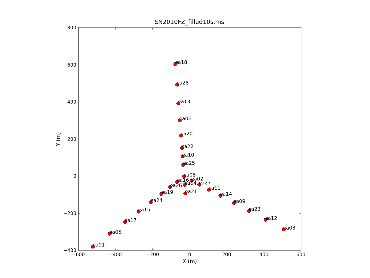
To plot up the antenna positions in the array:
# In CASA
plotants('SN2010FZ_filled10s.ms')
NOTE: if after this point or any other you get table locks, use clearstat to clear them:
# In CASA
clearstat
Now we examine the MS looking for bad data to flag. We will use plotms to bring up an interactive GUI that will display 2-D Y vs.X style line plots. NOTE: We do not recommend using the editing/flagging features of plotms. It is very easy to mess up your data that way. Also, we will be restricting the scope of plotting so most box/flag operations would not get rid of all the bad data. We will instead use plotms to identify bad data and then use flagcmd to flag it. This will also allow full scripting of the flagging.
WARNING: The Flag button on the plotms GUI is close to other buttons you will be using, in particular the one that gets rid of boxes you have drawn. Be careful and don't hit the Flag button by mistake!
The useful spw are 2~17. To get an idea of the data layout, plot a single baseline/channel versus time:
# In CASA
plotms(vis='SN2010FZ_filled10s.ms',field='',spw='2~17:31~31', \
       antenna='ea01&ea02',correlation='RR,LL',xaxis='time',yaxis='amp')

Look for bad antennas by picking the last field and plotting baselines versus antenna ea01:
# In CASA
plotms(vis='SN2010FZ_filled10s.ms',field='2',spw='2~17:31~31', \
       antenna='ea01',correlation='RR,LL',xaxis='antenna2',yaxis='amp')
You should be able to see that antenna 11 (= ea13) is bad (very low amplitude, it has no C-band receiver!) and that some of the spectral windows on 15 and 23 (ea17,ea25) are also on the low side. Boxing and using Locate will show that spw 10~17 are suspect for these antennas.
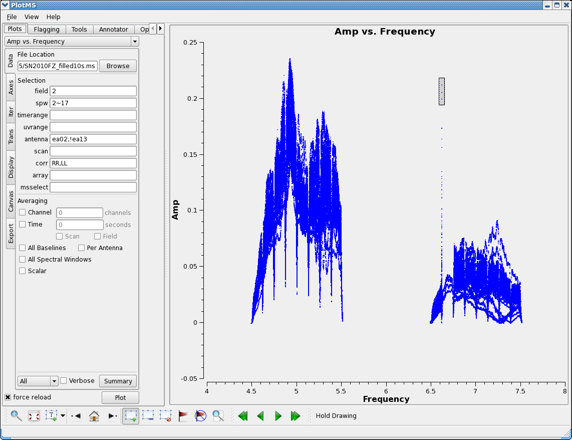
Now look at the bandpass for ea02 - it is in the inner core and a prospective reference antenna. Exclude ea13 using negation in the selection:
# In CASA
plotms(vis='SN2010FZ_filled10s.ms',field='2',spw='2~17', \
       antenna='ea02;!ea13',correlation='RR,LL',xaxis='frequency',yaxis='amp')
There is clearly less data for spw 11, and use of Locate shows spw 11 data only for ea02,ea03,04,08,09,11,12. We will later delete this incomplete spw. Note also the very strong RFI spike at 6614MHz (spw 10 ch 63) with clear ringing contaminating both spw 10 and 11. There is also a tremendous roll-off in spw 10. We will drop these spectral window when we process the data.
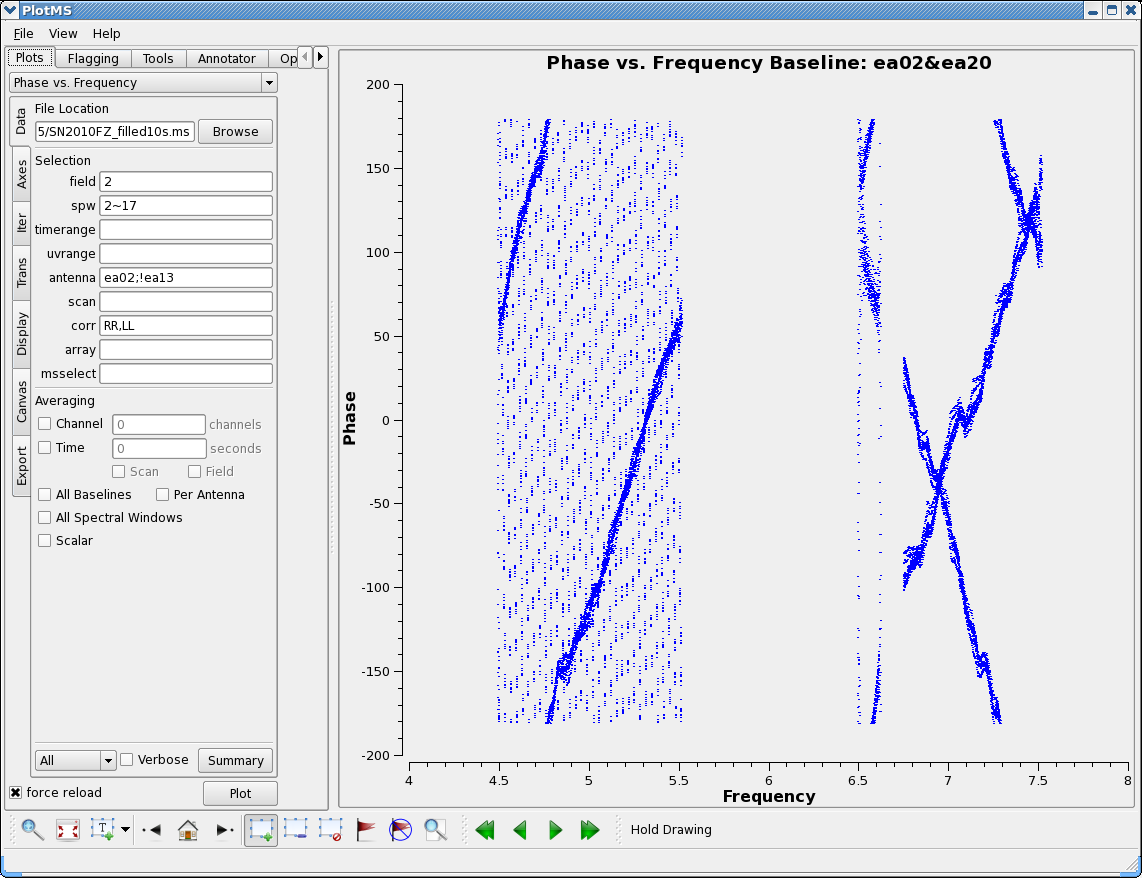
We can also step through the baselines to our antenna using iteraxis - use the ">" button to step through:
# In CASA
plotms(vis='SN2010FZ_filled10s.ms',field='2',spw='2~17',antenna='ea02;!ea13', \
       correlation='RR,LL',xaxis='frequency',yaxis='amp',iteraxis='baseline')
This will make it easier to isolate the bad antennas. Now plot the phases, iterating through baselines to ea02:
# In CASA
plotms(vis='SN2010FZ_filled10s.ms',field='2',spw='2~17',antenna='ea02;!ea13', \
       correlation='RR,LL',xaxis='frequency',yaxis='phase',iteraxis='baseline')
You see the slopes due to residual delays. Mostly a turn or less over a 128MHz subband, but there are some outliers. Step through to ea20. You see that there is a very large delay in RR (via locate) for the first baseband (spw 0~7). We will delete this (will also delete LL so there are no orphan polarization products). Note ea17 and ea25 baselines drop close to zero in the middle of upper baseband (e.g. plot 'ea17&ea25') so we will delete these.
To carry out flagging, we again use flagcmd in the mode where it takes a list of command strings:
# In CASA
flaglist = ['antenna="ea13"',
            'antenna="ea17" spw="10~17"',
            'antenna="ea25" spw="10~17"',
            'antenna="ea20" spw="2~9"']
flagcmd(vis='SN2010FZ_filled10s.ms',flagmode='cmd',command=flaglist,optype='apply',flagbackup=False)
These commands will be carried out as well as being added to the FLAG_CMD table (marked as applied).
Plot the data again now having flagged:
# In CASA
plotms(vis='SN2010FZ_filled10s.ms',field='2',spw='2~17',antenna='ea02', \
       correlation='RR,LL',xaxis='frequency',yaxis='amp',scan='7~44')
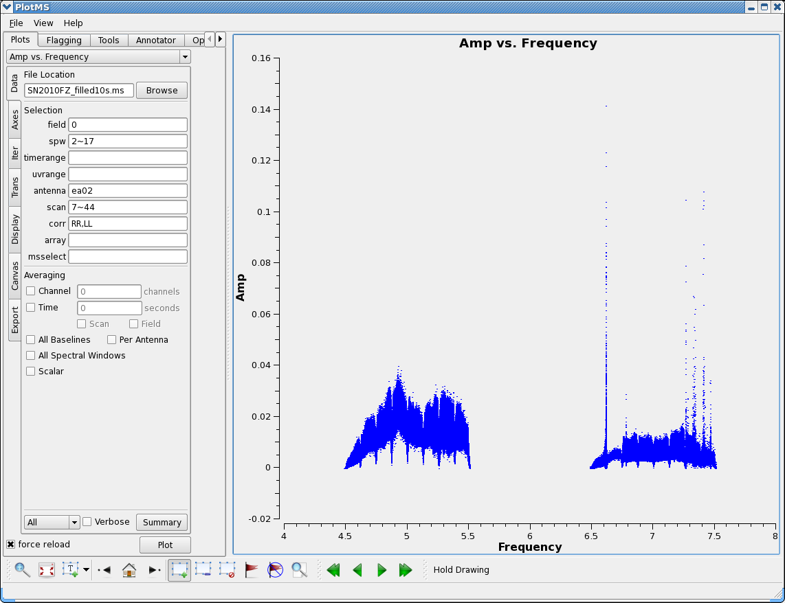
Now our phase calibrator - it is weaker, and we now start to see the RFI:
# In CASA
plotms(vis='SN2010FZ_filled10s.ms',field='0',spw='2~17',antenna='ea02', \
       correlation='RR,LL',xaxis='frequency',yaxis='amp',scan='7~44')
Use the Zoom feature, Mark rectangles and use Locate to identify the frequency/channel of RFI. In particular, we note in our analysis:
- 6614MHz (spw 10 ch 63) super strong
- 6772-6778MHz (spw 12 ch 14-17)
- 7260-7264MHz (spw 16 ch 2-4)
- 7314-7340MHz (spw 16 ch 29-42)
- 7402-7418MHz (spw 17 ch 9-17)
- 7458-7466MHz (spw 17 ch 37-41)
- 7488MHz (spw 17 ch 52)
If you plot all antennas and avoid the band edges you see spw 16,17 are pretty wiped out:
# In CASA
plotms(vis='SN2010FZ_filled10s.ms',field='0',spw='2~17:4~59',antenna='', \
       correlation='RR,LL',xaxis='frequency',yaxis='amp',scan='7~44')
For now we will not flag these channels but note them to mask out when creating continuum calibration tables and images.
Finally, split off the good scans and spw, this will allow us to work on the data without having to start completely over if we mess something up badly as well as letting us do simpler selection:
# In CASA
split(vis='SN2010FZ_filled10s.ms',outputvis='SN2010FZ_flagged10s.ms',datacolumn='data',spw='2~9,12~17',scan='7~44')
You now have a MS called SN2010FZ_flagged10s.ms in your working area. This should be 2.8GB in size.
Calibration
Summarize the split flagged MS:
# In CASA
listobs('SN2010FZ_flagged10s.ms')
In the logger we see:
================================================================================
           MeasurementSet Name:  /home/sandrock2/smyers/casa/tutorials/SN2010FZ/SN2010FZ_flagged10s.ms      MS Version 2
================================================================================
   Observer: Dr. Alicia M. Soderberg     Project: T.B.D.
Observation: EVLA
Data records: 1374548       Total integration time = 3042 seconds
   Observed from   11-Jul-2010/21:36:01.0   to   11-Jul-2010/22:26:43.0 (UTC)

   ObservationID = 0         ArrayID = 0
  Date        Timerange (UTC)          Scan  FldId FieldName nVis   Int(s)   SpwIds      ScanIntent
  11-Jul-2010/21:36:01.0 - 21:38:20.5     7      0 J0925+0019   73710  9.93     [0, 1, 2, 3, 4, 5, 6, 7, 8, 9, 10, 11, 12, 13]CALIBRATE_PHASE#UNSPECIFIED
              21:38:44.0 - 21:39:51.0     9      1 SN2010FZ     39312  9.11     [0, 1, 2, 3, 4, 5, 6, 7, 8, 9, 10, 11, 12, 13]OBSERVE_TARGET#UNSPECIFIED
              21:40:01.0 - 21:41:20.5    10      1 SN2010FZ     44226  9.89     [0, 1, 2, 3, 4, 5, 6, 7, 8, 9, 10, 11, 12, 13]OBSERVE_TARGET#UNSPECIFIED
              21:41:30.0 - 21:42:50.0    11      1 SN2010FZ     44226  10       [0, 1, 2, 3, 4, 5, 6, 7, 8, 9, 10, 11, 12, 13]OBSERVE_TARGET#UNSPECIFIED
              21:43:00.0 - 21:44:20.0    12      1 SN2010FZ     44226  10       [0, 1, 2, 3, 4, 5, 6, 7, 8, 9, 10, 11, 12, 13]OBSERVE_TARGET#UNSPECIFIED
              21:44:30.0 - 21:45:50.0    13      1 SN2010FZ     44226  10       [0, 1, 2, 3, 4, 5, 6, 7, 8, 9, 10, 11, 12, 13]OBSERVE_TARGET#UNSPECIFIED
              21:46:00.0 - 21:47:19.5    14      1 SN2010FZ     44226  9.89     [0, 1, 2, 3, 4, 5, 6, 7, 8, 9, 10, 11, 12, 13]OBSERVE_TARGET#UNSPECIFIED
              21:47:29.0 - 21:47:48.5    15      1 SN2010FZ     14742  9.67     [0, 1, 2, 3, 4, 5, 6, 7, 8, 9, 10, 11, 12, 13]OBSERVE_TARGET#UNSPECIFIED
              21:48:12.0 - 21:49:18.5    16      0 J0925+0019   39312  8.92     [0, 1, 2, 3, 4, 5, 6, 7, 8, 9, 10, 11, 12, 13]CALIBRATE_PHASE#UNSPECIFIED
              21:49:42.0 - 21:50:49.0    17      1 SN2010FZ     39312  9.11     [0, 1, 2, 3, 4, 5, 6, 7, 8, 9, 10, 11, 12, 13]OBSERVE_TARGET#UNSPECIFIED
              21:50:59.0 - 21:52:19.0    18      1 SN2010FZ     44226  10       [0, 1, 2, 3, 4, 5, 6, 7, 8, 9, 10, 11, 12, 13]OBSERVE_TARGET#UNSPECIFIED
              21:52:29.0 - 21:53:48.5    19      1 SN2010FZ     44226  9.89     [0, 1, 2, 3, 4, 5, 6, 7, 8, 9, 10, 11, 12, 13]OBSERVE_TARGET#UNSPECIFIED
              21:53:58.0 - 21:55:18.0    20      1 SN2010FZ     44226  10       [0, 1, 2, 3, 4, 5, 6, 7, 8, 9, 10, 11, 12, 13]OBSERVE_TARGET#UNSPECIFIED
              21:55:28.0 - 21:56:48.0    21      1 SN2010FZ     44226  10       [0, 1, 2, 3, 4, 5, 6, 7, 8, 9, 10, 11, 12, 13]OBSERVE_TARGET#UNSPECIFIED
              21:56:58.0 - 21:58:18.0    22      1 SN2010FZ     44226  10       [0, 1, 2, 3, 4, 5, 6, 7, 8, 9, 10, 11, 12, 13]OBSERVE_TARGET#UNSPECIFIED
              21:58:28.0 - 21:58:47.0    23      1 SN2010FZ     14742  9.33     [0, 1, 2, 3, 4, 5, 6, 7, 8, 9, 10, 11, 12, 13]OBSERVE_TARGET#UNSPECIFIED
              21:59:11.0 - 22:00:17.0    24      0 J0925+0019   39312  8.93     [0, 1, 2, 3, 4, 5, 6, 7, 8, 9, 10, 11, 12, 13]CALIBRATE_PHASE#UNSPECIFIED
              22:00:40.0 - 22:01:47.0    25      1 SN2010FZ     39312  9.12     [0, 1, 2, 3, 4, 5, 6, 7, 8, 9, 10, 11, 12, 13]OBSERVE_TARGET#UNSPECIFIED
              22:01:57.0 - 22:03:17.0    26      1 SN2010FZ     44226  10       [0, 1, 2, 3, 4, 5, 6, 7, 8, 9, 10, 11, 12, 13]OBSERVE_TARGET#UNSPECIFIED
              22:03:27.0 - 22:04:47.0    27      1 SN2010FZ     44226  10       [0, 1, 2, 3, 4, 5, 6, 7, 8, 9, 10, 11, 12, 13]OBSERVE_TARGET#UNSPECIFIED
              22:04:57.0 - 22:06:16.5    28      1 SN2010FZ     44226  9.89     [0, 1, 2, 3, 4, 5, 6, 7, 8, 9, 10, 11, 12, 13]OBSERVE_TARGET#UNSPECIFIED
              22:06:26.0 - 22:07:46.0    29      1 SN2010FZ     44226  10       [0, 1, 2, 3, 4, 5, 6, 7, 8, 9, 10, 11, 12, 13]OBSERVE_TARGET#UNSPECIFIED
              22:07:56.0 - 22:09:16.0    30      1 SN2010FZ     44226  10       [0, 1, 2, 3, 4, 5, 6, 7, 8, 9, 10, 11, 12, 13]OBSERVE_TARGET#UNSPECIFIED
              22:09:26.0 - 22:09:45.0    31      1 SN2010FZ     14742  9.33     [0, 1, 2, 3, 4, 5, 6, 7, 8, 9, 10, 11, 12, 13]OBSERVE_TARGET#UNSPECIFIED
              22:10:08.5 - 22:11:15.0    32      0 J0925+0019   39312  8.94     [0, 1, 2, 3, 4, 5, 6, 7, 8, 9, 10, 11, 12, 13]CALIBRATE_PHASE#UNSPECIFIED
              22:11:38.5 - 22:12:45.5    33      1 SN2010FZ     39312  9.11     [0, 1, 2, 3, 4, 5, 6, 7, 8, 9, 10, 11, 12, 13]OBSERVE_TARGET#UNSPECIFIED
              22:12:55.0 - 22:14:15.0    34      1 SN2010FZ     44226  10       [0, 1, 2, 3, 4, 5, 6, 7, 8, 9, 10, 11, 12, 13]OBSERVE_TARGET#UNSPECIFIED
              22:14:25.0 - 22:15:45.0    35      1 SN2010FZ     44226  10       [0, 1, 2, 3, 4, 5, 6, 7, 8, 9, 10, 11, 12, 13]OBSERVE_TARGET#UNSPECIFIED
              22:15:55.0 - 22:17:15.0    36      1 SN2010FZ     44226  10       [0, 1, 2, 3, 4, 5, 6, 7, 8, 9, 10, 11, 12, 13]OBSERVE_TARGET#UNSPECIFIED
              22:17:25.0 - 22:18:44.5    37      1 SN2010FZ     44226  9.89     [0, 1, 2, 3, 4, 5, 6, 7, 8, 9, 10, 11, 12, 13]OBSERVE_TARGET#UNSPECIFIED
              22:18:54.0 - 22:20:14.0    38      1 SN2010FZ     44226  10       [0, 1, 2, 3, 4, 5, 6, 7, 8, 9, 10, 11, 12, 13]OBSERVE_TARGET#UNSPECIFIED
              22:20:24.0 - 22:20:43.5    39      1 SN2010FZ     14742  9.6      [0, 1, 2, 3, 4, 5, 6, 7, 8, 9, 10, 11, 12, 13]OBSERVE_TARGET#UNSPECIFIED
              22:21:06.5 - 22:22:13.5    40      0 J0925+0019   38584  8.96     [0, 1, 2, 3, 4, 5, 6, 7, 8, 9, 10, 11, 12, 13]CALIBRATE_PHASE#UNSPECIFIED
              22:25:13.0 - 22:25:13.0    42      2 3C286        770    2.65     [0, 1, 2, 3, 4, 5, 6, 7, 8, 9, 10, 11, 12, 13]CALIBRATE_BANDPASS#UNSPECIFIED,CALIBRATE_AMPLI#UNSPECIFIED
              22:25:23.0 - 22:26:43.0    43      2 3C286        42812  9.62     [0, 1, 2, 3, 4, 5, 6, 7, 8, 9, 10, 11, 12, 13]CALIBRATE_BANDPASS#UNSPECIFIED,CALIBRATE_AMPLI#UNSPECIFIED
           (nVis = Total number of time/baseline visibilities per scan)
Fields: 3
  ID   Code Name         RA            Decl           Epoch   SrcId nVis
  0    D    J0925+0019   09:25:07.8150 +00.19.13.9334 J2000   0     230230
  1    NONE SN2010FZ     09:42:04.7700 +00.19.51.0000 J2000   1     1100736
  2    K    3C286        13:31:08.2880 +30.30.32.9589 J2000   2     43582
   (nVis = Total number of time/baseline visibilities per field)
Spectral Windows:  (14 unique spectral windows and 1 unique polarization setups)
  SpwID  #Chans Frame Ch1(MHz)    ChanWid(kHz)TotBW(kHz)  Ref(MHz)    Corrs
  0          64 TOPO  4488        2000        128000      4488        RR  RL  LR  LL
  1          64 TOPO  4616        2000        128000      4616        RR  RL  LR  LL
  2          64 TOPO  4744        2000        128000      4744        RR  RL  LR  LL
  3          64 TOPO  4872        2000        128000      4872        RR  RL  LR  LL
  4          64 TOPO  5000        2000        128000      5000        RR  RL  LR  LL
  5          64 TOPO  5128        2000        128000      5128        RR  RL  LR  LL
  6          64 TOPO  5256        2000        128000      5256        RR  RL  LR  LL
  7          64 TOPO  5384        2000        128000      5384        RR  RL  LR  LL
  8          64 TOPO  6744        2000        128000      6744        RR  RL  LR  LL
  9          64 TOPO  6872        2000        128000      6872        RR  RL  LR  LL
  10         64 TOPO  7000        2000        128000      7000        RR  RL  LR  LL
  11         64 TOPO  7128        2000        128000      7128        RR  RL  LR  LL
  12         64 TOPO  7256        2000        128000      7256        RR  RL  LR  LL
  13         64 TOPO  7384        2000        128000      7384        RR  RL  LR  LL
Sources: 42
  ID   Name         SpwId RestFreq(MHz)  SysVel(km/s)
  0    J0925+0019   0     -              -
  0    J0925+0019   1     -              -
  0    J0925+0019   2     -              -
  0    J0925+0019   3     -              -
  0    J0925+0019   4     -              -
  0    J0925+0019   5     -              -
  0    J0925+0019   6     -              -
  0    J0925+0019   7     -              -
  0    J0925+0019   8     -              -
  0    J0925+0019   9     -              -
  0    J0925+0019   10    -              -
  0    J0925+0019   11    -              -
  0    J0925+0019   12    -              -
  0    J0925+0019   13    -              -
  1    SN2010FZ     0     -              -
  1    SN2010FZ     1     -              -
  1    SN2010FZ     2     -              -
  1    SN2010FZ     3     -              -
  1    SN2010FZ     4     -              -
  1    SN2010FZ     5     -              -
  1    SN2010FZ     6     -              -
  1    SN2010FZ     7     -              -
  1    SN2010FZ     8     -              -
  1    SN2010FZ     9     -              -
  1    SN2010FZ     10    -              -
  1    SN2010FZ     11    -              -
  1    SN2010FZ     12    -              -
  1    SN2010FZ     13    -              -
  2    3C286        0     -              -
  2    3C286        1     -              -
  2    3C286        2     -              -
  2    3C286        3     -              -
  2    3C286        4     -              -
  2    3C286        5     -              -
  2    3C286        6     -              -
  2    3C286        7     -              -
  2    3C286        8     -              -
  2    3C286        9     -              -
  2    3C286        10    -              -
  2    3C286        11    -              -
  2    3C286        12    -              -
  2    3C286        13    -              -
Antennas: 27:
  ID   Name  Station   Diam.    Long.         Lat.
  0    ea01  W09       25.0 m   -107.37.25.2  +33.53.51.0
  1    ea02  E02       25.0 m   -107.37.04.4  +33.54.01.1
  2    ea03  E09       25.0 m   -107.36.45.1  +33.53.53.6
  3    ea04  W01       25.0 m   -107.37.05.9  +33.54.00.5
  4    ea05  W08       25.0 m   -107.37.21.6  +33.53.53.0
  5    ea06  N06       25.0 m   -107.37.06.9  +33.54.10.3
  6    ea08  N01       25.0 m   -107.37.06.0  +33.54.01.8
  7    ea09  E06       25.0 m   -107.36.55.6  +33.53.57.7
  8    ea10  N03       25.0 m   -107.37.06.3  +33.54.04.8
  9    ea11  E04       25.0 m   -107.37.00.8  +33.53.59.7
  10   ea12  E08       25.0 m   -107.36.48.9  +33.53.55.1
  11   ea13  N07       25.0 m   -107.37.07.2  +33.54.12.9
  12   ea14  E05       25.0 m   -107.36.58.4  +33.53.58.8
  13   ea15  W06       25.0 m   -107.37.15.6  +33.53.56.4
  14   ea16  W02       25.0 m   -107.37.07.5  +33.54.00.9
  15   ea17  W07       25.0 m   -107.37.18.4  +33.53.54.8
  16   ea18  N09       25.0 m   -107.37.07.8  +33.54.19.0
  17   ea19  W04       25.0 m   -107.37.10.8  +33.53.59.1
  18   ea20  N05       25.0 m   -107.37.06.7  +33.54.08.0
  19   ea21  E01       25.0 m   -107.37.05.7  +33.53.59.2
  20   ea22  N04       25.0 m   -107.37.06.5  +33.54.06.1
  21   ea23  E07       25.0 m   -107.36.52.4  +33.53.56.5
  22   ea24  W05       25.0 m   -107.37.13.0  +33.53.57.8
  23   ea25  N02       25.0 m   -107.37.06.2  +33.54.03.5
  24   ea26  W03       25.0 m   -107.37.08.9  +33.54.00.1
  25   ea27  E03       25.0 m   -107.37.02.8  +33.54.00.5
  26   ea28  N08       25.0 m   -107.37.07.5  +33.54.15.8
Note that the spws are re-numbered to 0-13.
Prepare the MS for calibration by adding scratch columns. This will take a few minutes.
# In CASA
clearcal('SN2010FZ_flagged10s.ms')
Setting the flux density scale
Before calibrating, we put a model for flux calibration source 3C286 into the MS (in the MODEL_DATA column we just created). Have it set the flux on a per-channel basis. NOTE: This uses the AOC Unix location for casapy models (yours may be different):
# In CASA
setjy(vis='SN2010FZ_flagged10s.ms',field='2',spw='',scalebychan=True, \
      modimage='/usr/lib64/casapy/data/nrao/VLA/CalModels/3C286_C.im')
It reports to logger that its about 7.7Jy at lower end to 5.7Jy at upper frequency limit.
Calibrating delays and bandpass
First, we do a phase-only calibration solution on a narrow range of channels in each spw on the bandpass/flux calibrator 3c286 to flatten them before solving for the bandpass. Note where we saw RFI in the higher spw and avoid those channels. The range 23~28 should work. Pick a refant near center - ea02 is a reasonable bet:
# In CASA
gaincal(vis='SN2010FZ_flagged10s.ms',caltable='calSN2010FZ.G0',field='2',spw='0~13:23~28', \
        gaintype='G',refant='ea02',calmode='p',solint='int',minsnr=3)
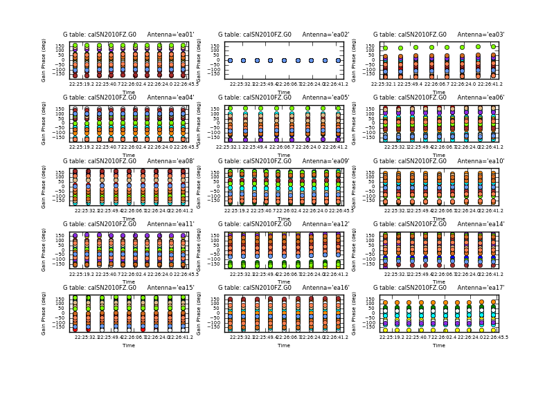
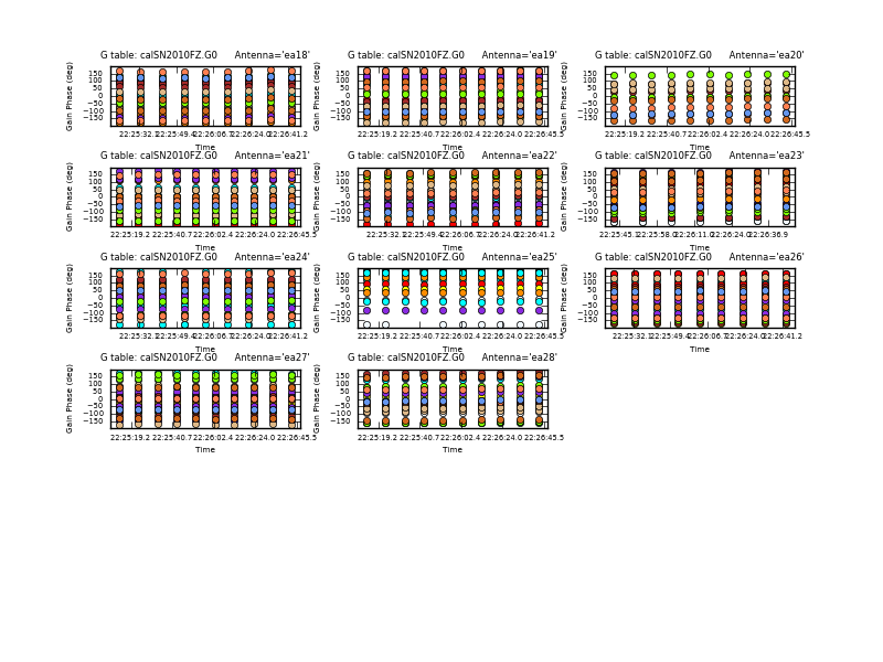
Plot the phase solutions (using full phase range instead of autorange)
# In CASA
plotcal(caltable='calSN2010FZ.G0',xaxis='time',yaxis='phase',iteration='antenna', \
        plotrange=[-1,-1,-180,180])
Step through the antenna-based solutions. They look good (and fairly flat over the scans). NOTE: If you want to make single-page multipanel plots (like those shown to the right), particularly for hardcopy (where it only shows the first page), you can do:
# In CASA
plotcal(caltable='calSN2010FZ.G0',xaxis='time',yaxis='phase', \
        antenna='0~10,12~15',subplot=531,iteration='antenna', \
        plotrange=[-1,-1,-180,180],showgui=False,fontsize=6.0, \
        figfile='plotSN2010FZ_plotcal_G0p1.png')
plotcal(caltable='calSN2010FZ.G0',xaxis='time',yaxis='phase', \
        antenna='16~26',subplot=531,iteration='antenna', \
        plotrange=[-1,-1,-180,180],showgui=False,fontsize=6.0, \
        figfile='plotSN2010FZ_plotcal_G0p2.png')
We can now solve for the residual antenna-based delays that we saw in phase vs. frequency. This uses the gaintype='K' option in gaincal (this is not documented but is available in Version 3.2.1). Note that this currently does not do a "global fringe-fitting" solution for delays, but instead does a baseline-based delay solution to all baselines to the refant, treating these as antenna-based delays. In most cases with high-enough S/N to get baseline-based delay solutions this will suffice.
# In CASA
gaincal(vis='SN2010FZ_flagged10s.ms',caltable='calSN2010FZ.K0',gaintable='calSN2010FZ.G0', \
        field='2',spw='0~13:4~59',gaintype='K', \
        refant='ea02',combine='scan',solint='inf',minsnr=3)
We pre-apply our initial phase table, and produce a new K-type caltable for input to bandpass calibration. The delays found are sent to the terminal. They are up to a few nanoseconds.
Now solve for the bandpass using the previous tables:
# In CASA
bandpass(vis='SN2010FZ_flagged10s.ms',caltable='calSN2010FZ.B0', \
         gaintable=['calSN2010FZ.G0','calSN2010FZ.K0'], \
         field='2',refant='ea02',solnorm=True, \
         bandtype='B', combine='scan', solint='inf')
Now plot this, in amplitude then phase:
# In CASA
plotcal(caltable='calSN2010FZ.B0',xaxis='freq',yaxis='amp',iteration='antenna')

plotcal(caltable='calSN2010FZ.B0',xaxis='freq',yaxis='phase',iteration='antenna', \
        plotrange=[-1,-1,-180,180])
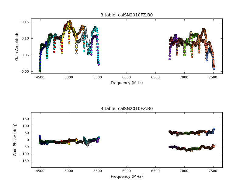
In the bandpass phase you no longer see the residual antenna delays but there are some band edge effects. Note that some antennas have a little strange bandpasses at upper end of lower baseband in spw 5,6,7 (e.g. ea14,ea16,ea17,ea25). To plot amp and phase for a single antenna versus frequency (see plots at right):
# In CASA
plotcal(caltable='calSN2010FZ.B0',xaxis='freq',yaxis='amp', \
        antenna='ea14',subplot=211,showgui=False, \
        figfile='')
plotcal(caltable='calSN2010FZ.B0',xaxis='freq',yaxis='phase', \
        antenna='ea14',subplot=212,showgui=False, \
        plotrange=[-1,-1,-180,180],figfile='plotSN2010FZ_plotcal_B0ea14.png')
Final phase and amplitude calibration
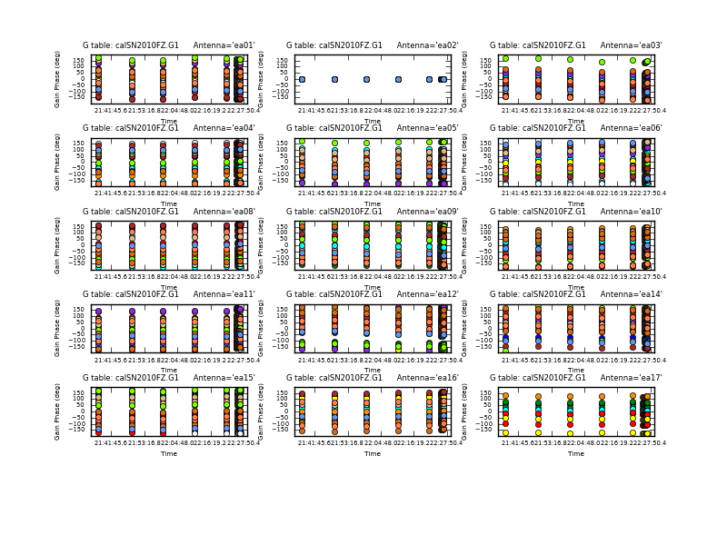
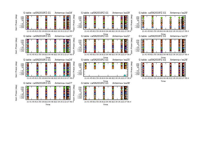
Now calibrate phases for real with wider bandwidth. First the flux calibrator again, with a per-integration solution time:
# In CASA
gaincal(vis='SN2010FZ_flagged10s.ms',caltable='calSN2010FZ.G1', \
        gaintable=['calSN2010FZ.K0','calSN2010FZ.B0'], \
        field='2',refant='ea02',solnorm=F, spw='0~13:4~59', \
        solint='int',gaintype='G',calmode='p')
Next our phase calibrator, appending these solutions to previous table. Exclude RFI channels here, and obtain one solution per scan:
# In CASA
gaincal(vis='SN2010FZ_flagged10s.ms',caltable='calSN2010FZ.G1',
        gaintable=['calSN2010FZ.K0','calSN2010FZ.B0'], \
        field='0',refant='ea02',solnorm=F, \
        spw='0:10~59,1~7:4~59,8:4~13;18~59,9~11:4~59,12:4~13;18~29;31~33;46~51;53~59,13:4~8;15~36;42~59', \
        solint='inf',gaintype='G',calmode='p',append=True)
The phases look reasonably connected:
# In CASA
plotcal(caltable='calSN2010FZ.G1',xaxis='time',yaxis='phase',iteration='antenna', \
        plotrange=[-1,-1,-180,180])
Now solve for amplitudes on a per scan interval. Do these separately using gainfield so phases don't get transferred across fields. Uses linear interpolation of the previously determined phases by default. Pre-apply the gaincurve also:
# In CASA
gaincal(vis='SN2010FZ_flagged10s.ms', caltable='calSN2010FZ.G2', \
        gaintable=['calSN2010FZ.K0','calSN2010FZ.B0','calSN2010FZ.G1'], \
        gainfield=['2','2','2'], field='2',refant='ea02',solnorm=F,
        spw='0:10~59,1~7:4~59,8:4~13;18~59,9~11:4~59,12:4~13;18~29;31~33;46~51;53~59,13:4~8;15~36;42~59', \
        solint='inf',gaintype='G',calmode='a',gaincurve=True)

gaincal(vis='SN2010FZ_flagged10s.ms', caltable='calSN2010FZ.G2', \
        gaintable=['calSN2010FZ.K0','calSN2010FZ.B0','calSN2010FZ.G1'],\
        gainfield=['2','2','0'], field='0',refant='ea02',solnorm=F, \
        spw='0:10~59,1~7:4~59,8:4~13;18~59,9~11:4~59,12:4~13;18~29;31~33;46~51;53~59,13:4~8;15~36;42~59', \
        solint='inf',gaintype='G',calmode='a',gaincurve=True,append=True)
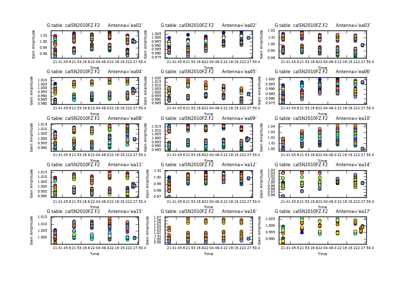
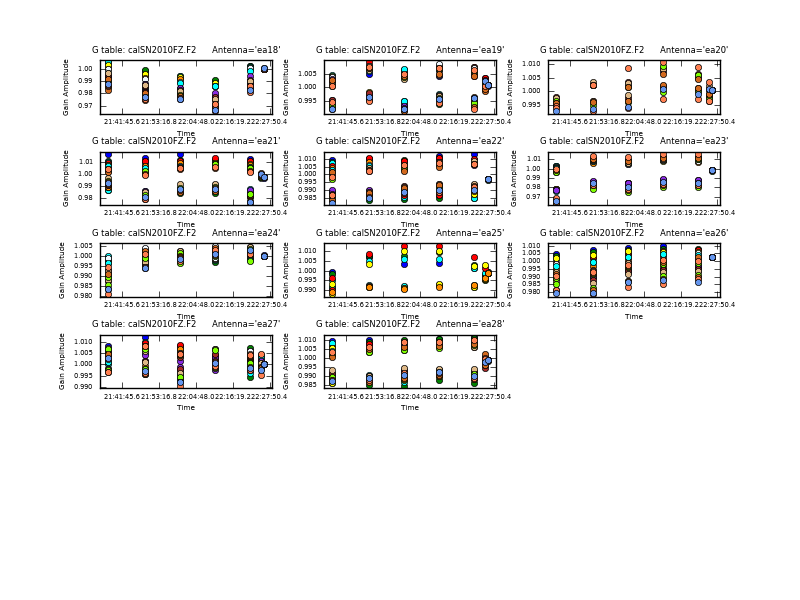
Since the flux on the gain calibrator is not scaled to its correct flux (but to 1.0Jy) use fluxscale to transfer the amplitude gains from 3c286:
# In CASA
fluxscale(vis='SN2010FZ_flagged10s.ms',caltable='calSN2010FZ.G2', \
          fluxtable='calSN2010FZ.F2',reference='2',transfer='0')
As it so happens, the derived flux for J0925+0019 is about 1 Jy and flat spectrum (you can plot up the raw amplitudes for fields 0,2 and convince yourself this is indeed true and not a bug). Plot these:
# In CASA
plotcal(caltable='calSN2010FZ.F2',xaxis='time',yaxis='amp',iteration='antenna')
The phase calibrator has consistent gains across the short run, though there is a slight offset to 3c286 (which is not nearby in any event).
Applying the Calibration and Final Editing
Next we actually apply all our accumulated calibration tables. We apply these to the calibration fields individually using the appropriate gainfields and interpolation for each:
# In CASA
applycal(vis='SN2010FZ_flagged10s.ms',field='2', \
         gaintable=['calSN2010FZ.K0','calSN2010FZ.B0','calSN2010FZ.G1','calSN2010FZ.F2'], \
         gainfield=['','','2','2'],interp=['nearest','nearest','linear','nearest'], \
         parang=False,calwt=F,gaincurve=T)

For the nearby calibrator we did only scan-based phase solutions so we use nearest interpolation:
# In CASA
applycal(vis='SN2010FZ_flagged10s.ms',field='0', \
         gaintable=['calSN2010FZ.K0','calSN2010FZ.B0','calSN2010FZ.G1','calSN2010FZ.F2'], \
         gainfield=['','','0','0'], interp=['nearest','nearest','nearest','nearest'], \
         parang=False,calwt=F,gaincurve=T)
Finally we apply calibration from field 0 to the target field 1. This takes a few minutes:
# In CASA
applycal(vis='SN2010FZ_flagged10s.ms',field='1', \
         gaintable=['calSN2010FZ.K0','calSN2010FZ.B0','calSN2010FZ.G1','calSN2010FZ.F2'], \
         gainfield=['','','0','0'], interp=['nearest','nearest','linear','linear'], \
         parang=False,calwt=F,gaincurve=T)
We can examine the corrected data on 3c286 using our RFI mask from above and avoiding band edges
# In CASA
plotms(vis='SN2010FZ_flagged10s.ms',field='2', \
       spw='0:10~59,1~7:4~59,8:4~13;18~59,9~11:4~59,12:4~13;18~29;31~33;46~51;53~59,13:4~8;15~36;42~59', \
       correlation='RR,LL',xaxis='frequency',yaxis='amp',ydatacolumn='corrected')
We now see problems in spw 5 and 6 for baseline ea17&ea25, which gives a really strange response:
# In CASA
plotms(vis='SN2010FZ_flagged10s.ms',field='2', \
       spw='0:10~59,1~7:4~59,8:4~13;18~59,9~11:4~59,12:4~13;18~29;31~33;46~51;53~59,13:4~8;15~36;42~59', \
       antenna='ea17&ea25', \
       correlation='RR,LL',xaxis='frequency',yaxis='amp',ydatacolumn='corrected')
You can exclude this through antenna negation:
# In CASA
plotms(vis='SN2010FZ_flagged10s.ms',field='2', \
       spw='0:10~59,1~7:4~59,8:4~13;18~59,9~11:4~59,12:4~13;18~29;31~33;46~51;53~59,13:4~8;15~36;42~59', \
       antenna='!ea17&ea25', \
       correlation='RR,LL',xaxis='frequency',yaxis='amp',ydatacolumn='corrected')
Then use Locate for the other bad points, which seem to indicate spw 5,6,7 for ea14,ea16,ea17,ea25. Exclude these and replot:
# In CASA
plotms(vis='SN2010FZ_flagged10s.ms',field='2', \
       spw='0:10~59,1~7:4~59,8:4~13;18~59,9~11:4~59,12:4~13;18~29;31~33;46~51;53~59,13:4~8;15~36;42~59', \
       antenna='!ea14;!ea16;!ea17;!ea25', \
       correlation='RR,LL',xaxis='frequency',yaxis='amp',ydatacolumn='corrected')

This now looks clean except for the RFI in the upper subbands.
Do flagging based on these:
# In CASA
flaglist = ['antenna="ea14,ea16,ea17,ea25" spw="5~7"']
flagcmd(vis='SN2010FZ_flagged10s.ms',flagmode='cmd',command=flaglist, \
        optype='apply',flagbackup=False)
Now replot the corrected data (you may have to force reload if you plotted same thing right before this):
# In CASA
plotms(vis='SN2010FZ_flagged10s.ms',field='2', \
       spw='0:10~59,1~7:4~59,8:4~13;18~59,9~11:4~59,12:4~13;18~29;31~33;46~51;53~59,13:4~8;15~36;42~59', \
       correlation='RR,LL',xaxis='frequency',yaxis='amp',ydatacolumn='corrected')
Looks good. If we were more diligent we would go back and recalibrate, but this looks good enough for now.
Plot the phase:
# In CASA
plotms(vis='SN2010FZ_flagged10s.ms',field='2', \
       spw='0:10~59,1~7:4~59,8:4~13;18~59,9~11:4~59,12:4~13;18~29;31~33;46~51;53~59,13:4~8;15~36;42~59', \
       correlation='RR,LL',xaxis='frequency',yaxis='phase',ydatacolumn='corrected')
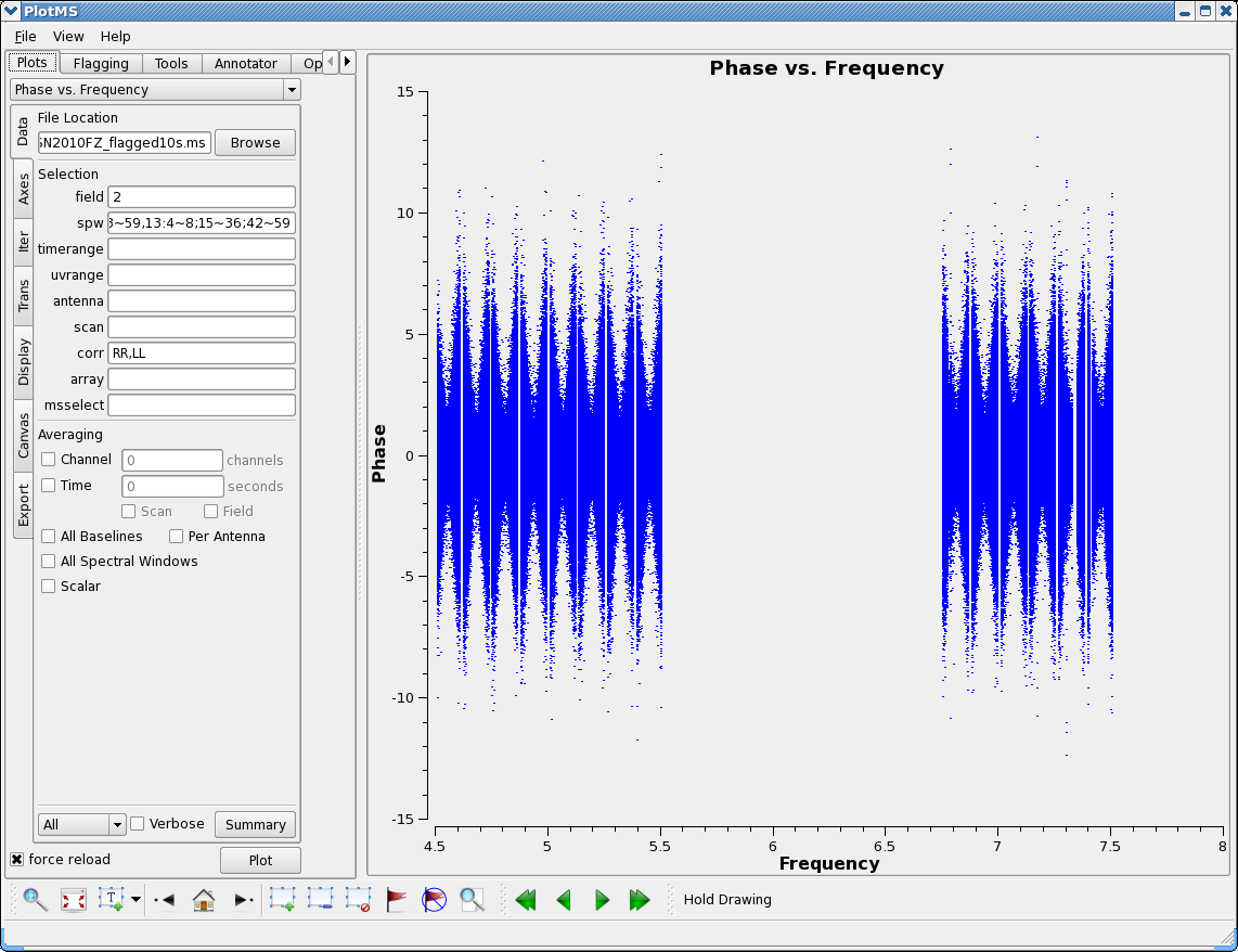
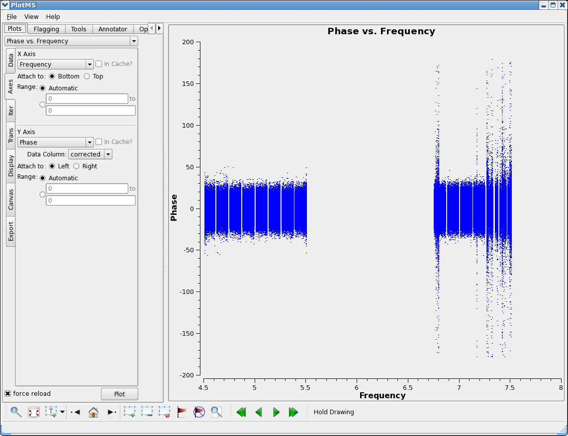
Note the characteristic "bowtie" pattern of the phases about the sub-band centers. Here we can see the effect of the EVLA "delay clunking", where the delay steps through discrete values such that the phase goes from -11deg to +11deg across the sub-band as the delay changes due to geometry. This is D-configuration so the delays change slowly, it will change faster in wider configurations. As of Q3 2011 we have not enabled the corrections for this in the EVLA system so you will always have this remaining delay error in your data. In principle you could solve for delays on short timescales and take this out, in practice this in not possible for your weaker target source in any event.
Now lets plot the corrected data amplitude for the phase calibrator:
# In CASA
plotms(vis='SN2010FZ_flagged10s.ms',field='0', \
       spw='0:10~59,1~7:4~59,8:4~13;18~59,9~11:4~59,12:4~13;18~29;31~33;46~51;53~59,13:4~8;15~36;42~59', \
       correlation='RR,LL',xaxis='frequency',yaxis='amp',ydatacolumn='corrected')
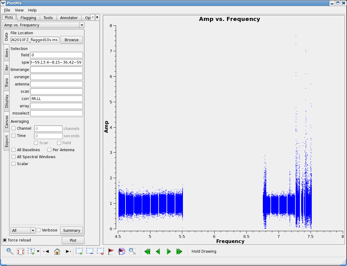
You can see the roll-off pumping up noise at the baseband edges (about 8-16 channels worth). Also, we can see some RFI we missed:
- <6804MHz spw 8 below ch 30 lots of bad stuff (alot from ea18,ea22 but others too)
- 7168MHz spw 11 ch 20
- pretty much all of spw 12,13
The ch 20 ones are all harmonics of the notorious 128MHz tone.
We will not flag these, but exclude them in imaging, so a good channel selection string for imaging might be:
spw = '0:16~59,1~6:4~59,7:4~54,8:30~59,9~10:4~59,11:4~19;21~59'
We can also plot the corrected phase - looks fairly good
# In CASA
plotms(vis='SN2010FZ_flagged10s.ms',field='0', \
       spw='0:10~59,1~7:4~59,8:4~13;18~59,9~11:4~59,12:4~13;18~29;31~33;46~51;53~59,13:4~8;15~36;42~59', \
       correlation='RR,LL',xaxis='frequency',yaxis='phase',ydatacolumn='corrected')
We can average over baseline and each scan:
# In CASA
plotms(vis='SN2010FZ_flagged10s.ms',field='0', \
       spw='0:10~59,1~7:4~59,8:4~13;18~59,9~11:4~59,12:4~13;18~29;31~33;46~51;53~59,13:4~8;15~36;42~59', \
       correlation='RR,LL',avgbaseline=True,avgtime='600s',
       xaxis='frequency',yaxis='phase',ydatacolumn='corrected')
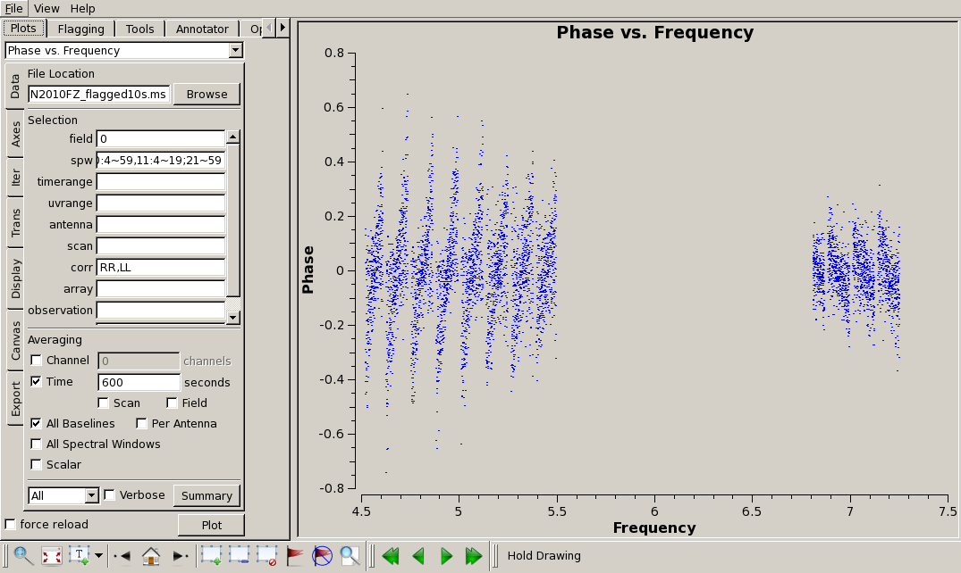
In this case we can see the residual effect of the EVLA "delay clunking" described above. It is reduced due to the averaging that we applied, but it is still there.
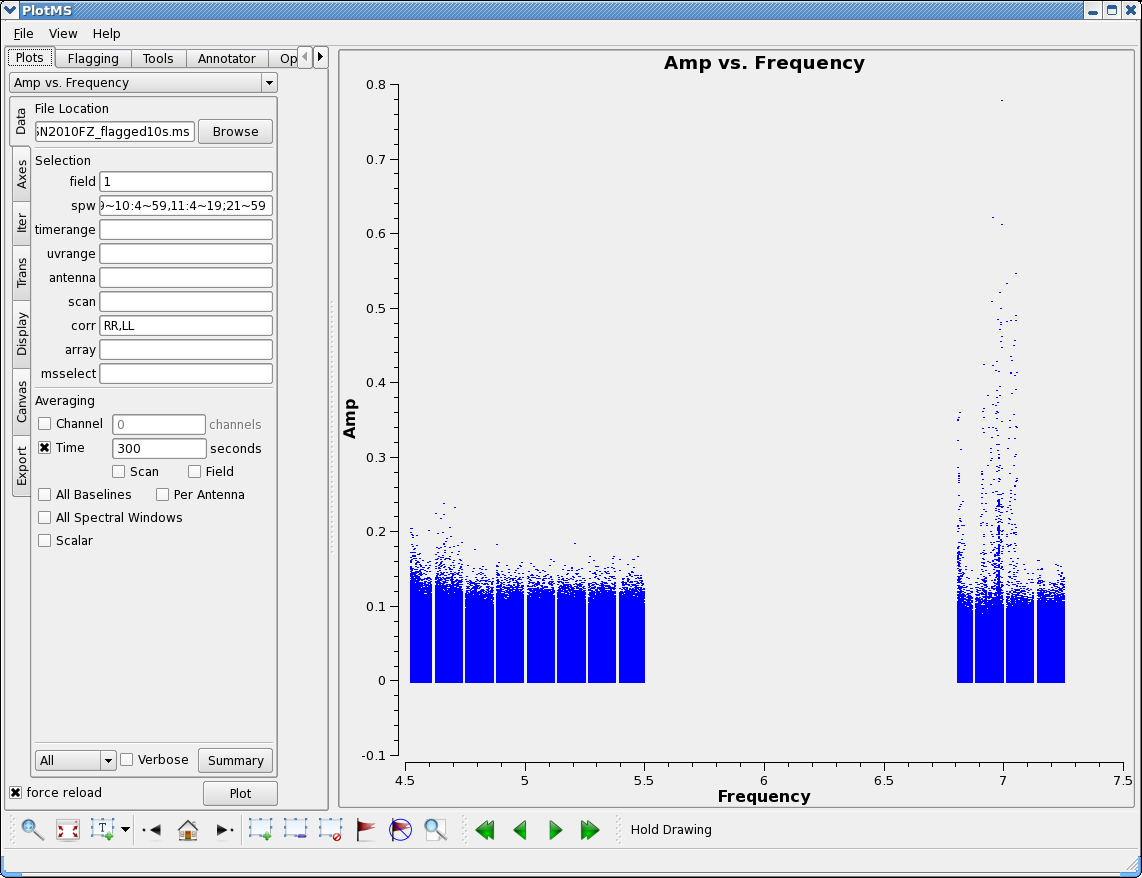
You can look at the target source field='1' but there are lots of data so you will need to do alot of averaging. For example:
# In CASA
plotms(vis='SN2010FZ_flagged10s.ms',field='1',avgtime='300s', \
       spw='0:16~59,1~6:4~59,7:4~54,8:30~59,9~10:4~59,11:4~19;21~59', \
       correlation='RR,LL',xaxis='frequency',yaxis='amp',ydatacolumn='corrected')
Alas, the upper baseband still has lots of low level RFI.
Now split off the data for calibrators and target, to avoid later issues that can corrupt the MSes. These will take a bit of time...field 1 took 18min on my workstation.
# In CASA
split(vis='SN2010FZ_flagged10s.ms',outputvis='SN2010FZ_split10s.ms',datacolumn='corrected',field='1')

split(vis='SN2010FZ_flagged10s.ms',outputvis='SN2010FZ_3c28610s.ms',datacolumn='corrected',field='2')

split(vis='SN2010FZ_flagged10s.ms',outputvis='SN2010FZ_J092510s.ms',datacolumn='corrected',field='0')
Imaging
This is D-config data at C-band, look at the Obs Status Summary: [1] Synthesized beam should be 12" at 6GHz with primary beam FOV 7.5arcmin (450"). Our data spans 4.5-7.5GHz : beam 9.6 at 7.5GHz and FOV 10' at 4.5GHz A cellsize of 3" should work, with an imsize > 200 to cover 2xFWHM FOV An imsize of 400+ will put the main beam inside the inner quarter safely The Briggs robust (0.5) weighting is somewhere between uniform and natural and will give reasonable resolution but still see some larger scale structure.
Due to the numerology of FFTW (which clean uses underneath for FFTs) optimal sizes, imsize should be composite number with two and only two prime factors chosen from 2,3,5. Taking into account the x1.2 padding that clean uses internally to the imsize you give it (and 1.2=2*3/5), we choose 640 or 1280 as our imsize (640=2^7*5). Other reasonable sets would be 405,1215,etc. (405=3^4*5) or 432,648,1296 (these are 2^n*3^m*5). In practice, if you give it non-optimal values for imsize, you may find that the transforms take a bit longer, which is noticeable if you are doing interactive clean.
Lets interactively clean one of the lower baseband spw (5): NOTE: this first time will take a few minutes at start to create scratch columns in the MS in case we want to do self-calibration later.
Cleaning a single spectral window

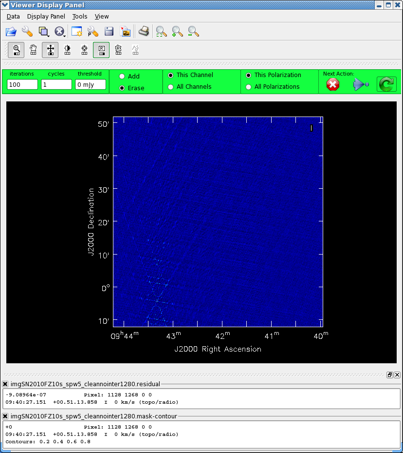
Start carefully by boxing the bright source and setting iterations to 10 at first Gradually add more boxes and increase the number of iterations Since this is not much more than a snapshot you see the six-fold sidelobe pattern of the extended emission in the center of the map. This decreases as you clean out this emission.
Stop cleaning when the residuals look like noise (and you cannot clearly see sources). To stop click the red X button.
# In CASA
clean(vis='SN2010FZ_split10s.ms',spw='5:4~59', \
      imagename='imgSN2010FZ10s_spw5_clean640', \
      mode='mfs',nterms=1,niter=10000,gain=0.1,threshold='0.0mJy', \
      psfmode='clark',imsize=[640,640],cell=['3.0arcsec'],stokes='I', \
      imagermode='csclean', cyclefactor=1.5, \
      weighting='briggs',robust=0.5,calready=True,interactive=True)
The top figure to the right shows a zoom in on the end state of the clean, where we have marked a number of boxes and cleaned them out.
Note that there are some strange sidelobe patterns in lower left, possibly from a source outside the image area. We can make a bigger image starting from our current model:
# In CASA
clean(vis='SN2010FZ_split10s.ms',spw='5:4~59', \
      imagename='imgSN2010FZ10s_spw5_clean1280', \
      mode='mfs',nterms=1,niter=10000,gain=0.1,threshold='0.0mJy', \
      psfmode='clark',imsize=[1280,1280],cell=['3.0arcsec'],stokes='I', \
      imagermode='csclean', cyclefactor=1.5, \
      modelimage='imgSN2010FZ10s_spw5_clean640.model', \
      weighting='briggs',robust=0.5,calready=True,interactive=True)
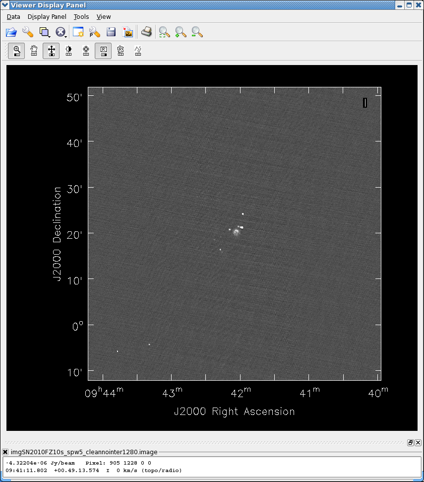
Sure enough, there is a bright source near the lower left (see middle panel at right). Box it, clean it a bit, and look again. There is a second source in the mid-left (track it down by its sidelobes). Box this one, clean it a bit, and when satisfied stop.
# In CASA
viewer('imgSN2010FZ10s_spw5_clean1280.image')
The restored image is shown in bottom panel to the right. I have chosen the Grayscale1 instead of default color map as I prefer grayscale to false color for assessing image quality. Check the rms of the residuals using the imstat task:
# In CASA
mystat = imstat('imgSN2010FZ10s_spw5_clean1280.residual')
print 'Residual standard deviation = '+str(mystat['sigma'][0])
I got 31.8uJy for mine.
Cleaning the lower baseband
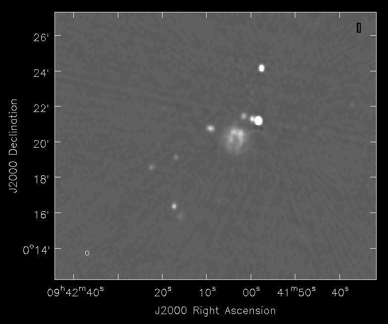
Now, image the entire lower baseband (spw 0-7). Follow same iterative procedure as before, and get the best residuals you can. Because of the bandwidth and frequency synthesis, the sidelobe pattern is different than before and it is much easier to see fainter emission. Be careful cleaning sources that lie near or on sidelobe splotches. Clean the central emission region way down first to reduce the sidelobe level before adding components in the sidelobe areas.
# In CASA
clean(vis='SN2010FZ_split10s.ms',spw='0:16~59,1~6:4~59,7:4~54', \
      imagename='imgSN2010FZ10s_spw0to7_clean1280', \
      mode='mfs',nterms=1,niter=10000,gain=0.1,threshold='0.0mJy', \
      psfmode='clark',imsize=[1280,1280],cell=['3.0arcsec'],stokes='I', \
      imagermode='csclean', cyclefactor=1.5, \
      weighting='briggs',robust=0.5,calready=True,interactive=True)

mystat = imstat('imgSN2010FZ10s_spw0to7_clean1280.residual')
print 'Residual standard deviation = '+str(mystat['sigma'][0])
I got 11.3uJy (and there is clearly structure left in the residual). To the right is a zoom-in on the center of the restored image.


Lets try adding a spectral slope to the multi-frequency synthesis using nterms=2 on the lower baseband. This will solve for images of the average and spectral slope simultaneously. The dirty beam will have lower sidelobes so we turn up cyclefactor for csclean a bit:
# In CASA
clean(vis='SN2010FZ_split10s.ms',spw='0:16~59,1~6:4~59,7:4~54', \
      imagename='imgSN2010FZ10s_spw0to7_mfs2_clean1280', \
      mode='mfs',nterms=2,niter=10000,gain=0.1,threshold='0.0mJy', \
      psfmode='clark',imsize=[1280,1280],cell=['3.0arcsec'],stokes='I', \
      imagermode='csclean', cyclefactor=4.5, \
      weighting='briggs',robust=0.5,calready=True,interactive=True)

mystat = imstat('imgSN2010FZ10s_spw0to7_mfs2_clean1280.residual.tt0')
print 'Residual standard deviation = '+str(mystat['sigma'][0])
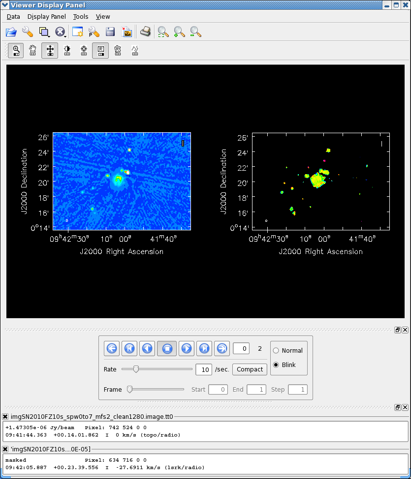
I got 10.5uJy (somewhat better looking than the nterms=1). The top screenshot to the right shows an intermediate but early stage of cleaning where we are looking at the central emission and cleaning it out slowly.
Cleaning the lower baseband using two MFS Taylor terms
The mfs nterms=2 option creates two "Taylor Term" images - an average intensity image (with suffix .image.tt0) and a spectral slope image (with suffix .image.tt1) which is intensity x alpha (where alpha is spectral index). For convenience there is a spectral index image (with suffix .image.alpha). These Taylor expansions are with respect to the "Reference Frequency" of the image (by default the center frequency of the spw selected, but can be specified using the reffreq parameter in clean). The convention for spectral index alpha is that
[math]\displaystyle{ S \propto \nu^\alpha }[/math]
so negative spectral indexes indicate a "steep" spectrum (falling with frequency).
You can use the viewer to load the average intensity
# In CASA
viewer('imgSN2010FZ10s_spw0to7_mfs2_clean1280.image.tt0')
and then use the Open Data panel to load imgSN2010FZ10s_spw0to7_mfs2_clean1280.image which can then be blinked (optionally plotted side-by-side using the Panel Display Options panel to set 2 panels in the x direction). Note there is lots of noise in the low-intensity regions, and thus filtering the alpha image based on the values in the tt0 image is desirable.
You can use the immath task to make this filtered alpha image explicitly, using a Lattice Expression Language (LEL) expression:
# In CASA
immath(imagename=['imgSN2010FZ10s_spw0to7_mfs2_clean1280.image.alpha',
                  'imgSN2010FZ10s_spw0to7_mfs2_clean1280.image.tt0'],
       mode='evalexpr',
       expr='IM0[IM1>5.0E-5]',
       outfile='imgSN2010FZ10s_spw0to7_mfs2_clean1280.image.alpha.filtered')
This will use 50uJy (or 5 x the sigma we found) as the cutoff. You can then view or manipulate the filtered alpha image as normal.
We can also use LEL to filter the alpha image on the intensity on-the-fly when we load this raster in the Open Data panel by specifying a LEL string in the LEL box instead of selecting the image from the directory listing. The LEL string:
'imgSN2010FZ10s_spw0to7_mfs2_clean1280.image.alpha'['imgSN2010FZ10s_spw0to7_mfs2_clean1280.image.tt0'>5.0E-05]
will replicate what we did above. The middle figure to the right shows the Open Data panel with our LEL string in it. Just click the Raster button to load this.
The lower panel to the right shows the intensity and LEL-filtered alpha images side-by-side in the viewer, zoomed in on the galaxy emission. Mousing over the alpha shows spectral indexes ranging from -1 to +1 in the center, with the brightest emission with alpha -0.7 in the knots in the disk.
Cleaning using both basebands combined
For the ultimate image, use the "clean" part of the upper baseband in addition to the lower (use spw 0-11). We will use mfs with nterms=2 (if you try nterms=1 on this wide bandwidth you will get much poorer residuals).
# In CASA
clean(vis='SN2010FZ_split10s.ms', \
      spw='0:16~59,1~6:4~59,7:4~54,8:30~59,9~10:4~59,11:4~19;21~59', \
      imagename='imgSN2010FZ10s_spw0to11_mfs2_clean1280', \
      mode='mfs',nterms=2,niter=10000,gain=0.1,threshold='0.0mJy', \
      psfmode='clark',imsize=[1280,1280],cell=['3.0arcsec'],stokes='I', \
      imagermode='csclean', cyclefactor=4.5, \
      weighting='briggs',robust=0.5,calready=True,interactive=True)

mystat = imstat('imgSN2010FZ10s_spw0to11_mfs2_clean1280.residual.tt0')
print 'Residual standard deviation = '+str(mystat['sigma'][0])
I got 8.2uJy.
Look at this in the viewer:
# In CASA
viewer('imgSN2010FZ10s_spw0to11_mfs2_clean1280.image.tt0')
Zoom in on the center:
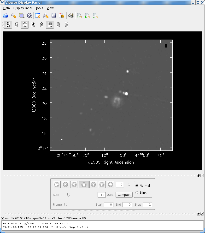
As a comparison, here is our image side by side with a i-band image from the Sloan Digital Sky Survey (SDSS) registered to our image:
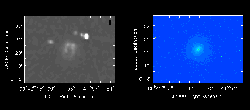
You can find this image and load it into your viewer, and blink against our 6cm image.
What to do next: some exercises for the user
Here are a number of things you can try after completing this tutorial:
- Use self-calibration to improve the data and re-clean to make a better image.
- Use multi-scale clean by adding non-zero scales to the multiscale parameter.
- Image the calibrators. What sort of dynamic range can you get on them? Is self-calibration needed (and if so what dynamic range do you get when you use it)?
- Try the testautoflag task (in 3.3.0 and later) to automatically flag RFI from the upper sideband.