Einstein-Face (CASA 3.2)

Simulations using non-science images: the face of Einstein

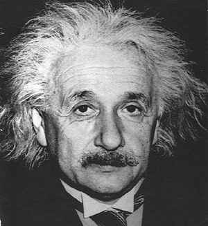
Simdata can be used to simulate any digitized image. These toy models can be particularly useful for examining the effects of varying uv-coverage on image fidelity if the "truth" model is a familiar object or image. In this example (which is on page 13 of the ALMA Early Science Primer)we use the face of Albert Einstein.

Step 1: obtain your image. Typically from the internet.

In this case, it is a jpg file.

Step 2: Convert your image to FITS

Various software programs have conversion to FITS enabled. The (GIMP) was used in this case. A handy list of FITS conversion programs is maintained by GSFC here

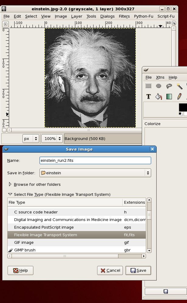
For the GIMP, start up the software

>gimp &

and in the main window select "Open" from the "File" menu.

The image will open up in a new window, you can use the GIMP to modify the image (adjust contrast, colormap etc).

Then, select "Save as" from the "File" menu in the window containing the image, and hit "Select File Type" in the dialog box to bring up the file type options, and select "Flexible Image Transport System". Pick a name for your file ending in .fits, e.g. einstein.fits

Step 3: check your file

Read your file into e.g. ds9to check that a valid FITS file has been produced. You can also examine the pixel values to examine the scaling of the image. In this case, Einstein's forehead has pixel values around 230 and the background around 40, so there is plenty of contrast. You can also examine the image header in ds9. Under the "File" menu, select "Display FITS Header" and examine the output. Make sure that SIMPLE = T, NAXIS=2 and check BITPIX. In this case, BITPIX=8, which is not valid for reading into CASA, so we need to change that at the next step.

FITS header produced by GIMP:

SIMPLE = T

BITPIX = 8

NAXIS = 2

NAXIS1 = 300

NAXIS2 = 327

BZERO = 0.000000

BSCALE = 1.000000

DATAMIN = 0.000000

DATAMAX = 255.000000

HISTORY THIS FITS FILE WAS GENERATED BY GIMP USING FITSRW

COMMENT FitsRW is (C) Peter Kirchgessner (peter@kirchgessner.net), but available

COMMENT under the GNU general public licence.

COMMENT For sources see http://www.kirchgessner.net

COMMENT Image type within GIMP: GIMP_GRAY_IMAGE

END

Step 4 Add FITS header keywords and change the format

At this stage, we need to perform some manipulations on the FITS file to get it readable by CASA. For convenience, we are also adding a WCS at this point (though this can also be done in simdata). This routine is written in IDL, using the IDL astronomy library, but similar manipulations can be carried out in IRAF, or using the python PyWCS and PyFITS libraries, available from the astropython project.

The IDL script is in File:Make 2dimage.pro.txt (remove the .txt from the filename before using).

IDL>make_2dimage,'einstein.fits',0,299,27,326

The IDL code performs the following manipulations:

1) Reads in the FITS file as a 2D array, trims it to 300x300 pixels and converts it to real, 300x300x1 array (the third dimension is added for generality to allow the construction of an image cube, it is not actually necessary in this particular case).

2) Creates header keywords corresponding to the axis types (CTYPE1,2,3) values at the reference pixels (CRVAL1,2,3), the reference pixel positions (CRPIX1,2,3) and the axis increments (CDELT1,2,3), and the epoch (EPOCH).

3) Writes out the modified FITS file as "twodmodel.fits"

Step 5 Start CASA and prepare inputs for simdata

Start with the 10min full science observation:

>casapy

default 'simdata'
project = 'fs_cfg8_10m'
modifymodel = F
skymodel = 'twodmodel.fits'
setpointings = T
integration = '300s'
mapsize = ['1arcmin','1arcmin']
maptype = 'hexagonal'
pointingspacing = '1arcmin'
predict = T

Antenna configuration: ALMA antenna configuration files are stored in a directory that depends on your CASA installation to be sure of finding them, identify the CASAPATH variable using the os.getenv command, and pick the configuration you want. Details on configuration choices are given in the [[1] M51 simulation guide].

repodir=os.getenv("CASAPATH").split(' ')[0]
antennalist        =  repodir+"/data/alma/simmos/alma.out08.cfg"
refdate = '2012/05/21/22:00:00' 
totaltime = '600s'
thermalnoise = ""
image = T
vis = '$project.ms'
imsize = [300,300]
cell = '0.043arcsec'
niter = 2000
weighting = 'natural'
analyze=F
simdata

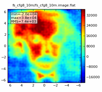
The output image should have a synthesized beam of 0.62"x0.56" and look something like:

Now we repeat for an 1hr observation:

tget simdata
project = 'fs_cfg8_1hr'
totaltime = '3600s'
simdata

Which should look something like: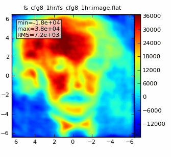

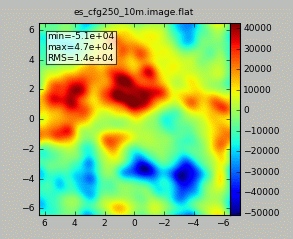
Finally, two Early Science simulations, using the 250m configuration. One 10min simulation:

tget simdata
project = 'es_cfg250_10m'
antennalist = repodir+"/data/alma/simmos/alma.early.250m.cfg"
totaltime = '600s'
simdata

which looks like this:

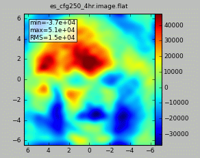
and a 4hr simulation:

tget simdata
project = 'es_cfg250_4hr'
totaltime = '14400s'
simdata

which looks like this:

Further experiments:

Some more things to try:

An 8hr observation shows the improvement obtained by obtaining fuller uv-coverage in the full science array:

tget simdata
antennalist = repodir+"/data/alma/simmos/alma.out08.cfg"
project = 'fs_cfg8_8hr'
totaltime = '28800s'
simdata

Which should look something like: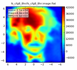

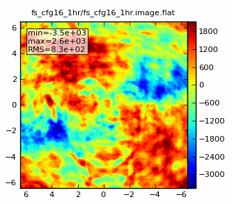
An attempt to make a higher resolution image shows what happens when short spacings are missing in the configuration. Configuration 16 has a 0.17x0.15 beam, still better than Nyquist sampling of the model image (which has 0.043" pixels). However, the lack of short spacings in the configuration leads to poorly sampled structure on large spatial scales. In practice, one would need to combine these observations with a set in a more compact configuration (such as 8) to sample both the large and small spatial structures.

tget simdata
antennalist = repodir+"/data/alma/simmos/alma.out16.cfg"
project = 'fs_cfg16_1hr'
totaltime = '3600s'
simdata

The result is: