Sunspot Band6 Feathering for CASA 6.5.4

Last checked on CASA Version 6.5.4

Overview

This guide features CARTA, the “Cube Analysis and Rendering Tool for Astronomy,” which is the new NRAO visualization tool for images and cubes. The CASA viewer (imview) has not been maintained for a few years and will be removed from future versions of CASA. We strongly recommend using CARTA, as it provides a much more efficient, stable, and feature rich user experience. A comparison of the CASA viewer and CARTA, as well as instructions on how to use CARTA at NRAO, is provided in the CARTA section of the CASA docs.

This portion of the Sunspot Band6 guide covers the combination process between the synthesized solar image and the full-sun image obtained with the TP array. It is the final step after:

1. calibrating the IF visibility data
2. imaging the IF data
3. calibrating and imaging the single-dish data

If you wish, you may skip parts 1 and 2, download the calibrated data package, Sunspot_Band6_CalibratedData.tgz, and complete part 3.

If you completed parts 1 and 2, we assume that you are working in the directory Sunspot_Band6_UncalibratedData. If you skip parts 1 and 2, and use the provided calibrated data, we assume that the working directory is Sunspot_Band6_CalibratedData.

Prepare the Single-Dish Data for Combination

List the Image Header

We start by defining names for our images.

# In CASA
if_base       = 'AR12470_B6AllSpw_I'                         # basename of the interferometric image
sd_base       = 'uid___A002_Xae00c5_X2e6b.PM03.StkI.Spw3'    # basename of the single dish image
combined_base = 'AR12470_B6AllSpw_I_Feather'                 # basename of the combined products

Now let's examine the single dish image header with imhead and mode='list'.

# In CASA
imhead(imagename=sd_base+'.rescl', mode='list')

Output are the supported keywords and their values in the format hdkey: hdvalue.

General --
        -- imtype: Intensity
        -- object: Sun
        -- equinox: J2000
        -- date-obs: 2015/12/18/20:12:21.416250
        -- observer: lknee
        -- projection: SIN
        -- restfreq: [248000000000.1]
        -- reffreqtype: LSRK
        -- telescope: ALMA
        -- beammajor: 26.722411arcsec
        -- beamminor: 26.722411arcsec
        -- beampa: 0deg
        -- bunit: K
        -- masks: [mask0]
        -- shape: [800, 800, 1, 1]
        -- datamin: 83.8561
        -- datamax: 7369.92
        -- minpos: 17:44:43.874 -23.04.42.909 I 2.4799e+11Hz
        -- minpixpos: [244, 770, 0, 0]
        -- maxpos: 17:43:24.017 -23.17.12.723 I 2.4799e+11Hz
        -- maxpixpos: [611, 520, 0, 0]
axes --
        -- ctype1: Right Ascension
        -- ctype2: Declination
        -- ctype3: Stokes
        -- ctype4: Frequency
crpix --
        -- crpix1: 400.0
        -- crpix2: 400.0
        -- crpix3: 0.0
        -- crpix4: 0.0
crval --
        -- crval1:  266.02.29.400deg.min.sec
        -- crval2: - 23.23.13.143deg.min.sec
        -- crval3: ['I']
        -- crval4: 247990336130.1Hz
cdelt --
        -- cdelt1: -  0.00.03.000deg.min.sec
        -- cdelt2:    0.00.03.000deg.min.sec
        -- cdelt3: 1
        -- cdelt4: 1999922065.6Hz
units --
        -- cunit1: rad
        -- cunit2: rad
        -- cunit3: 
        -- cunit4: Hz

Convert the Brightness Unit

Fig. 1.
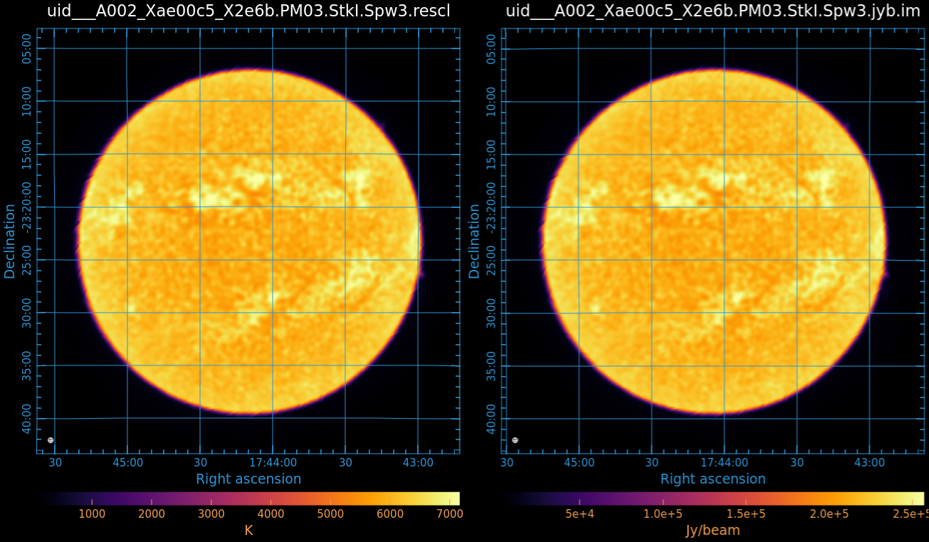
Left: The full-sun map with its original coordinate grid and brightness units of Kelvin.
Right: The shifted coordinate grid and brightness converted to units of Jy/beam.

The unit of the full-sun map is Kelvin. On the other hand, the unit of the synthesized image is Jy/beam. We retrieve frequency and beam size information with imhead, then convert the brightness values from K to Jy/beam with immath. This will produce a new image with the scaled values.

# In CASA

# derive a scaling factor based on single dish frequency and beam size
freq_SD   = imhead(sd_base+'.rescl', mode='get', hdkey='crval4')['value']
sd_bmajor = imhead(sd_base+'.rescl', mode='get', hdkey='beammajor')['value']
sd_bminor = imhead(sd_base+'.rescl', mode='get', hdkey='beamminor')['value']

convK2Jb = str(13.6 * (300./(freq_SD/1.e9))**2. * (1./sd_bmajor)*(1./sd_bminor))
# = '0.02787151811741245'

# create a new image with scaled values
import os
os.system(f'rm -rf {sd_base}.jyb.im')

immath(
  imagename=sd_base+'.rescl',
  expr='IM0/'+convK2Jb,
  outfile=sd_base+'.jyb.im')

# change the brightness unit in the new image header from K to Jy/beam
imhead(
  imagename=sd_base+'.jyb.im',
  mode='put',
  hdkey='bunit',
  hdvalue='Jy/beam')

Obtain the RA/Dec Coordinate of the Sun Center at the Reference Time

Before starting the combination process in CASA, we need to know the RA/Dec coordinate of the sun center at the reference time, which is used during the interferometric observation, because the observing time of the TP-array is not exactly the same. The Sun was moving on the RA/Dec coordinate frame during the gap between these observations. We need to shift the coordinate of the full-sun image based on the coordinate of the sun center at the reference time. The reference time of the observation is:
19:49:00UT, December 18 2015.

We obtain the RA/Dec coordinate of the sun center estimated from JPL's HORIZONS system:
RA: 266.01898 degree
Dec: -23.38648 degrees.

Change the Coordinate

RA/Dec are shown in the image header as ctype1/ctype2, which correspond to crval1/crval2. We shift the coordinate based on the RA/Dec coordinate obtained in the previous section by using mode='put' as follows.

# In CASA
import numpy as np
sun_ra = str(266.01898 * np.pi/180.)
sun_dec = str(-23.38648 * np.pi/180.)

imhead(imagename=sd_base+'.jyb.im', mode='put', hdkey='crval1', hdvalue=sun_ra)
imhead(imagename=sd_base+'.jyb.im', mode='put', hdkey='crval2', hdvalue=sun_dec)

The result of the process is shown in Figure 1. The look of the image has not changed, but the coordinates and units are now changed to match the synthesized image.

Regrid, Trim, and Primary Beam Correct

Fig. 2.
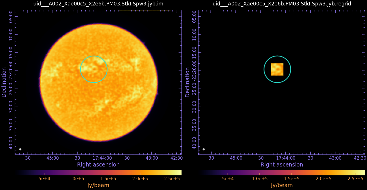
Left: The original full-sun image.
Right: The full-sun image regridded based on the synthesized image.

The images are spatially matched and raster scaling matched. A circular region is drawn to clearly show the spatial matching.

Fig. 3.
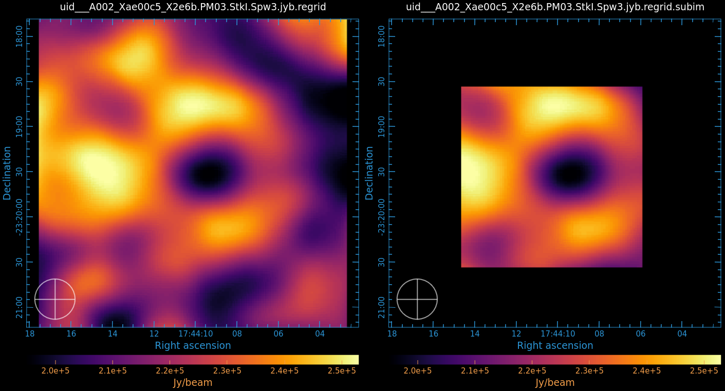
Left: The regridded full-sun image.
Right: The regridded image after trimming.

The images are spatially matched and raster scaling matched.

Now we regrid and trim the full-sun image with imregrid and imsubimage to match the size of the synthesized image as shown in Figure 2.

# In CASA
os.system(f'rm -rf {sd_base}.jyb.regrid')
os.system(f'rm -rf {sd_base}.jyb.regrid.subim')

imregrid(
  imagename=sd_base+'.jyb.im',
  template=if_base+'.image',
  axes=[0,1],
  output=sd_base+'.jyb.regrid')

imsubimage(
  imagename=sd_base+'.jyb.regrid',
  outfile=sd_base+'.jyb.regrid.subim',
  box='100,100,400,400')

Fig. 4.
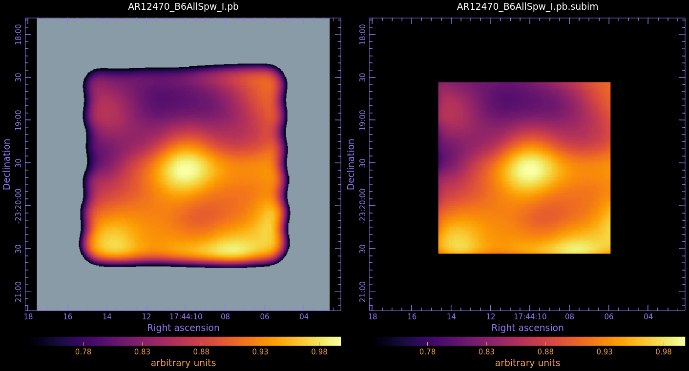
Left: The original primary beam used in synthesis imaging.
Right: The synth PB after trimming.

In CARTA, Preferences > Render Configuration > NaN color has been chosen as gray here to show that the dimension of the original includes the area outside of the primary beam cutoff of 0.73.

Fig. 5.
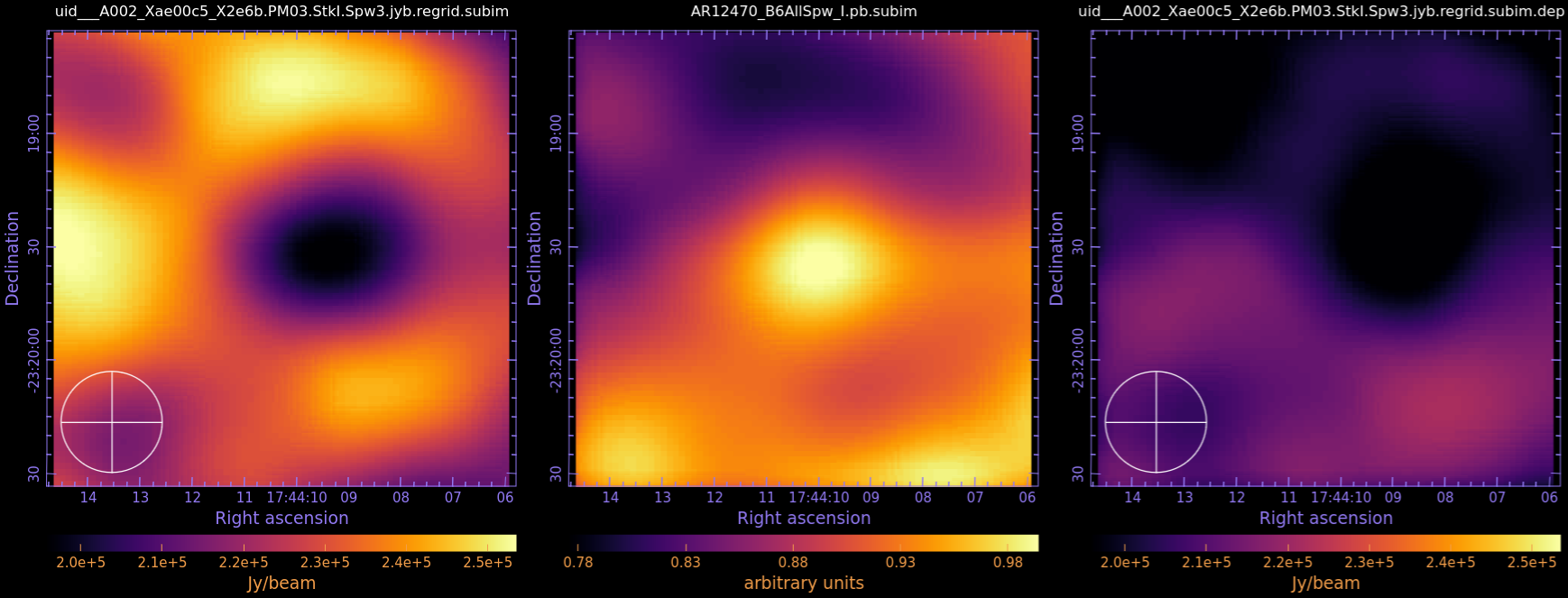
Left: The regridded and trimmed single dish image from Figure 3.
Center: The trimmed synth primary beam from Figure 4.
Right: The product of multiplying the first two, resulting in a regridded, trimmed, and PB corrected single dish image to match the synth image.

All three have been spacially matched, and the left and right are raster scaling matched. Note the color scale of each.

Finally, we trim the primary beam response of the synthesized image, and with immath we multiply this by the trimmed single-dish image:

# In CASA
os.system(f'rm -rf {if_base}.pb.subim')
os.system(f'rm -rf {sd_base}.jyb.regrid.subim.depb')

imsubimage(
  imagename=if_base+'.pb',
  outfile=if_base+'.pb.subim',
  box='100,100,400,400')

immath(
  imagename=[sd_base+'.jyb.regrid.subim',
             if_base+'.pb.subim'],
  expr='IM0*IM1',
  outfile=sd_base+'.jyb.regrid.subim.depb',
  imagemd=sd_base+'.jyb.regrid.subim')

We specify imagemd so that the header metadata, including units of Jy/beam and the RA/Dec coordinate we just set, is carried over from the single dish image instead of the trimmed synth primary beam.

Prepare the Synthesized Image for Combination

Fig. 6.
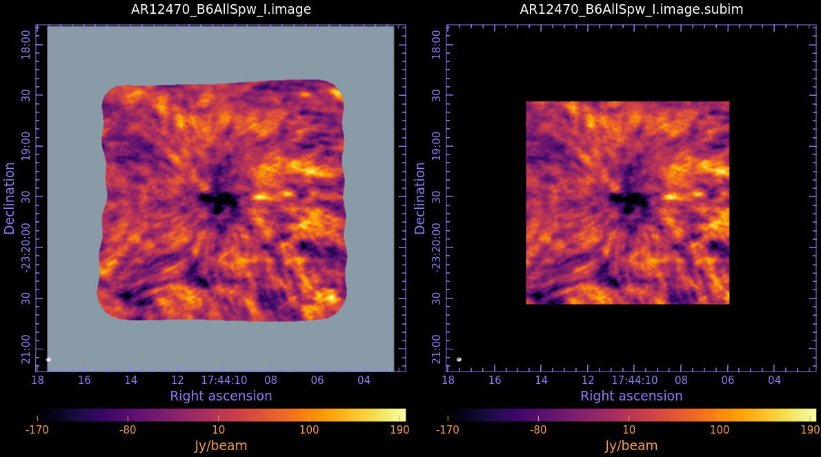
Left: The original synth image.
Right: The trimmed synth image.

We set the NaN color to gray to clearly show the dimensions of the original image including the area outside the PB cutoff.

Trim the synthesized image to fit the area of the trimmed single-dish image:

# In CASA
os.system(f'rm -rf {if_base}.image.subim')

imsubimage(
  imagename=if_base+'.image',
  outfile=if_base+'.image.subim',
  box='100,100,400,400')

Combination and Primary Beam Correction

Fig. 7.
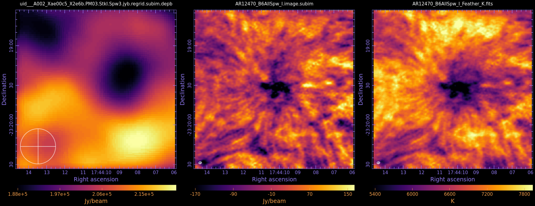
Left: The regridded, trimmed, and PB corrected single dish image from Figure 5.
Center: The trimmed synth image from Figure 6.
Right: The final combined single dish + synth image, PB corrected, converted to K, and exported to fits format.

The combination of the images can be done using feather, the same as for non-solar data.

# In CASA
os.system(f'rm -rf {combined_base}.image')

feather(
  imagename=combined_base+'.image',
  highres=if_base+'.image.subim',
  lowres=sd_base+'.jyb.regrid.subim.depb',
  sdfactor=1.0)

CAUTION: In this tutorial and the packages of the solar SV data released on 2017/01/18, we use the default parameters of the task, as shown above. As a result, the averaged brightness temperature of the combined image is always a few % larger than the brightness temperature at the same position in the single-dish map, although the values have to be the same. This means that you need to tune the sdfactor parameter of the task to obtain consistent images before using combined images for your science. See more details in the Image Combination section of the CASA Docs.

After the feathering process, we do the primary beam correction with impbcor as follows:

# In CASA
os.system(f'rm -rf {combined_base}.pbcor')

impbcor(
  imagename=combined_base+'.image',
  pbimage=if_base+'.pb.subim',
  outfile=combined_base+'.pbcor',
  mode='divide')

To convert the unit from Jy/beam to Kelvin, we use the following commands with imhead and immath.

# In CASA

# derive a scaling factor based on interferometric frequency and feather beam size
freq_IF  = imhead(if_base+'.image', mode='get', hdkey='crval4')['value']
f_bmajor = imhead(combined_base+'.image', mode='get', hdkey='beammajor')['value']
f_bminor = imhead(combined_base+'.image', mode='get', hdkey='beamminor')['value']

convJb2K = str(13.6 * (300./(freq_IF/1.e9))**2. * (1./f_bmajor)*(1./f_bminor))
# = '5.629310261438283'

# create a new image with scaled values
os.system(f'rm -rf {combined_base}_K.pbcor')

immath(
  imagename=combined_base+'.pbcor',
  expr='IM0*'+convJb2K,
  outfile=combined_base+'_K.pbcor')
  
# change the brightness unit in the new image header from Jy/beam to K 
imhead(
  imagename=combined_base+'_K.pbcor',
  mode='put',
  hdkey='bunit',
  hdvalue='K')

Finally, we create the FITS file of the combined and primary corrected map with exportfits.

# In CASA
os.system(f'rm -rf {combined_base}_K.fits')

exportfits(
  imagename=combined_base+'_K.pbcor',
  fitsimage=combined_base+'_K.fits')

The result of the combining is shown in Figure 7.

---

Caution: The single-dish images and feathering images in the solar SV data packages (ex. Sunspot_Band6_ReferenceImages.tgz) were not applied the re-scaling to the single-dish data (see Sunspot_Band6_SingleDish_for_CASA_6.5.4#Calibration_.28re-scaling.29_after_Imaging). Please do not use the reference image for your science.